One example of a tensor data set that shows up in most people's everyday lives is a series of images, or a movie. Each frame of a movie contains a horizontal axis and a vertical axis and can be considered a matrix where the elements are the pixel intensities. We stack the frames one on top of the other to form a tensor. Each element of this tensor is the intensity of a pixel at horizontal position \(i\), vertical position \(j\), and frame \(t\). I illustrate this "frame stacking" with the movie below:

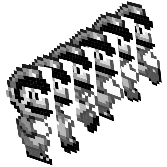
As seen in the far right, we might observe data that has been corrupted by noise --- that is, we see a fuzzy movie. The goal is to recover the uncorrupted movie. Denote the original movie by \(\Theta\). It is natural to model the noise as additive residual variation
\[ \mathcal{X} \overset{d}{=} \Theta + \mathcal{E}, \] where \(\mathcal{E}\) is the error tensor. Common schemes for estimating \(\Theta\) begin by first "vectorizing" each frame and then combining these vectorized images into one big matrix.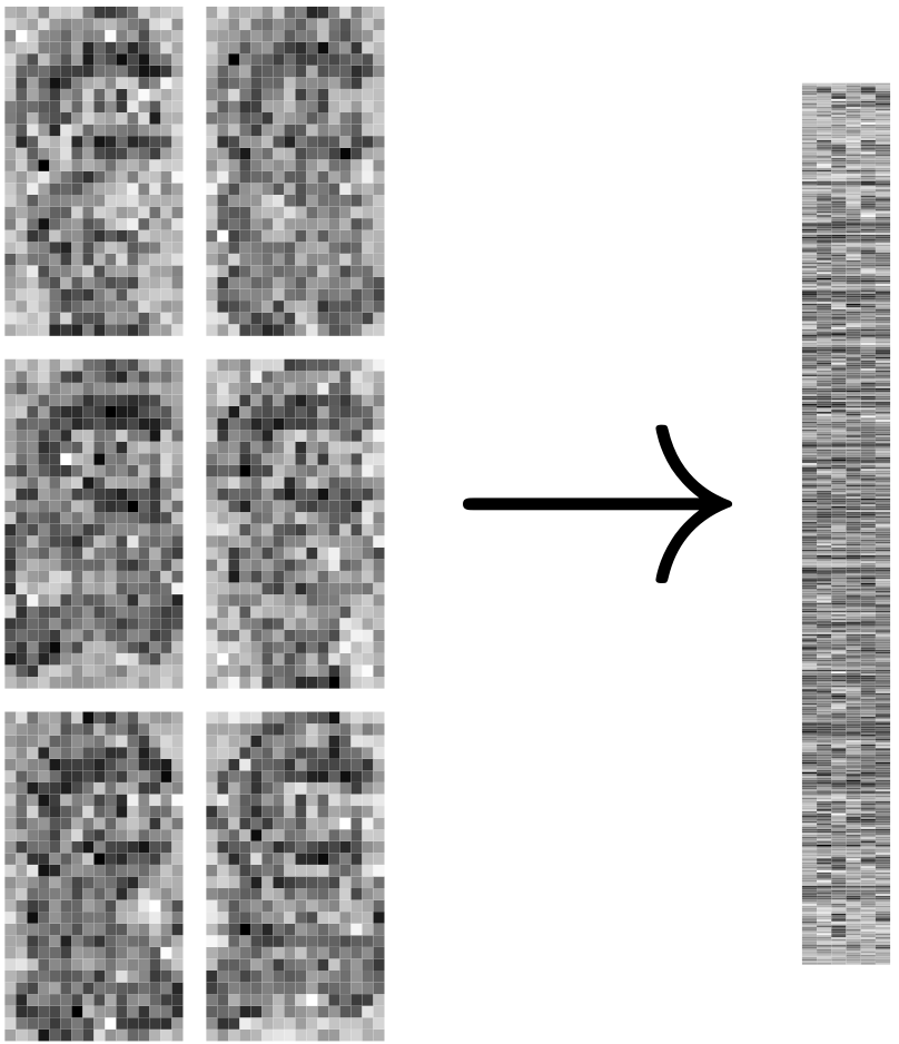
After this transformation, we perform some estimation scheme on this new matrix --- sometimes called a "Casorati" matrix --- and then "re-arrayicize" the estimate to obtain the "de-noised" movie. Since each frame of a movie is usually not too different from adjacent frames, we would expect a lot of co-linearity among the columns of this Casorati matrix. That is, this matrix is approximately low rank. Well performing estimators shrink toward this low rank structure, usually through the singular value decomposition (SVD). Let \(Y\) be the Casorati matrix. The SVD decomposes \(Y \in\mathbb{R}^{p\times n}\) into the product of three matrices \[ Y = UDV^T, \] where \(U\) and \(V\) have orthonormal columns and \(D = \text{diag}(\sigma_1,\ldots,\sigma_p)\) is a diagonal matrix such that \(\sigma_1 \geq \cdots\geq \sigma_p \geq 0\). The columns of \(U\) and \(V\) are called the left and right singular vectors, respectively, of \(Y\). The diagonal elements of \(D\) are the singular values. A key property of the SVD is that the number of non-zero singular values is exactly the rank of \(Y\). One way to shrink toward low rank structure, then, is to shrink the singular values toward zero. One can see an example of this approach in Candès el. al. [2013].
However, the first step in this estimation process was to destroy the tensor structure of the movie by converting it to a matrix. If we believe that there is tensor structure --- e.g. because vertically and horizontally adjacent pixels tend to have similar intensities --- then we can improve our estimators by shrinking toward this additional tensor-specific structure.
There is reason to believe that there is additional tensor structure here. The Casorati matrix indexes the time dimension along the columns and the two spatial dimensions along the rows. But there are other ways to convert a tensor to a matrix. We may construct a matrix where the columns index the x-axis and the rows index both the time and the y-axis dimensions. We may also construct a matrix where the columns index the y-axis and the rows index the time and x-axis dimensions. Below are scree-plots (plots of the singular values) for these three matrices:
Each matrix seems to be well-approximated by a rank 1 matrix. Shrinking toward the space of tensors that are simultaneously low rank in each of these "matricizations" seems like it should improve the estimation of \(\Theta\). Developing estimators that accomplish this was my third project with Peter Hoff and you can read about it in Gerard and Hoff [2017]. Specifically, we looked at the higher-order SVD of De Lathauwer et. al. [2000]: \[ \mathcal{X} = (U_1,\ldots,U_K)\cdot\mathcal{S}, \] where the \(U_k\)'s contain orthonormal columns and \(\mathcal{S}\) is the "core" tensor having the same dimension as \(\mathcal{X}\). The "\(\cdot\)" denotes multilinear multiplication, or the Tucker product. Shrinking this \(\mathcal{S}\) is the tensor-analogue to shrinking the singular values in the matrix case, and results in estimators that are (approximately) low rank along each matricization.
We have to be a little clever about how we perform this shrinkage, though. It's not at first clear what type of shrinkage and how much shrinkage should be performed to this \(\mathcal{S}\) tensor. We ultimately decided on estimators of the form \[ t(\mathcal{X}) = (U_1,\ldots,U_K)\cdot(f_1(D_1),\ldots,f_K(D_K))\cdot(D_1^{-1},\ldots,D_K^{-1})\cdot\mathcal{S}, \] where each \(D_k\) contains the mode-specific singular values of each matricization of \(\mathcal{X}\), and each \(f_k(\cdot)\) maps a diagonal matrix to another diagonal matrix. Writing the estimators in this way allows us to (1) shrink toward low rank structure along all matricizations through the Tucker product and (2) allows us to use the mode-specific singular values to determine the amount of shrinkage to perform along each dimension. These \(f_k(\cdot)\)'s usually contain tuning parameters, though, whose choice is usually difficult. We proposed using an unbiased estimate of the mean squared error to choose these tuning parameters.
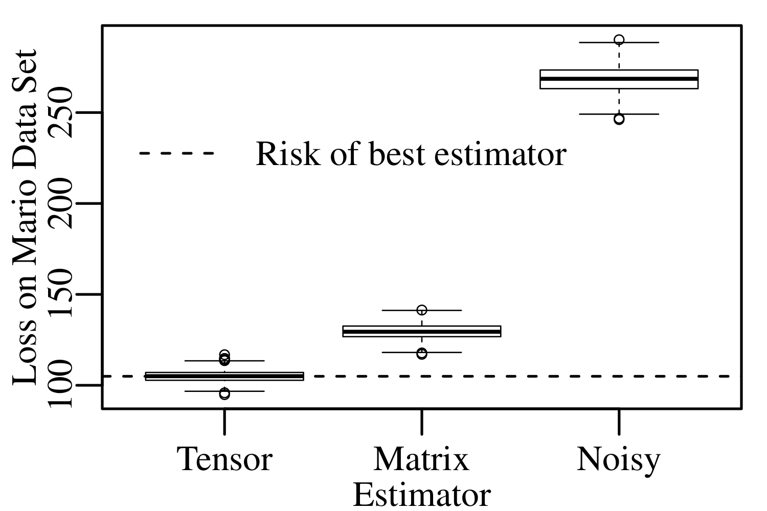
To demonstrate the applicability of our approach, we generated 1000 noisy Mario movies and calculated our estimator and a matrix-specific shrinkage estimator for each of these movies. We then calculated the squared error loss. When we compared our estimator against the matrix specific estimator on the noisy Mario movie, ours won handily:
References
Gerard, D., & Hoff, P. (2017). Adaptive higher-order spectral estimators. Electronic Journal of Statistics, 11(2), p. 3703–3737. doi:10.1214/17-EJS1330 | arXiv:1505.02114
Candès, E. J., Sing-Long, C. A., & Trzasko, J. D. (2013). Unbiased risk estimates for singular value thresholding and spectral estimators. IEEE transactions on signal processing, 61(19), p. 4643-4657 doi:10.1109/TSP.2013.2270464
De Lathauwer, L., De Moor, B., & Vandewalle, J. (2000). A multilinear singular value decomposition. SIAM journal on Matrix Analysis and Applications, 21(4), p. 1253-1278. doi:10.1137/S0895479896305696