My buddy Felipe has started to get me interested in these organisms called “polyploids.” Humans are “diploid”, meaning that they have two copies of their DNA (“di” = Greek for two). As such, a lot of methods in statistical genetics assume that an organism has two copies of its DNA. However, lots of interesting organisms (particularly in agriculture, like wheat, potatoes, blueberries, sugarcane, and strawberries) have more than two copies of their DNA. And so they are “polyploids” (“poly” = Greek for many).
I wanted to tackle a fundamental task in statistical genetics in the context of polyploid organisms: Genotyping. A first step in lots of bioinformatics pipelines is to detect and quantify the differences in the DNA between different organisms. This step is called “genotyping”. One type of difference that can occur in DNA is a single nucleotide polymorphism (SNP), where at a single location on the DNA we see a different character (or nucleotide — one of A, T, G, or C) between different individuals in the population. Usually, individuals will only have one of two types of differences (or “alleles”) at a single SNP. People in the literature often denote one allele by an “A” (one of A, T, G, or C) and the other allele by an “a” (again, one of A, T, G, or C).
To do the genotyping, we will consider a specific biological assay, Genotyping by Sequencing (GBS). GBS consists of the following steps:
- (i) Chop up (or “digest”) the genome of an individual into small bits (or “reads”).
- (ii) Make many copies of (or “amplify”) these reads.
- (iii) Sequence all of these small reads so that we know what nucleotides are on each read.
- (iv) Locate where on a reference genome each of these reads belongs (this step is called “mapping”).
- (v) What we ultimately have is the number of small reads at a SNP which have one allele (A) and the number of reads at the same SNP which have the other allele (a).
As you can see, biology is not for want of jargon: “ploidy”, “genotyping”, “SNP”, “allele”, “nucleotide”, “read”, “digest”, “amplify”, “map”, “sequence”.
Well, it’s something you get used to.
I’ve graphically depicted the steps involved in GBS below:
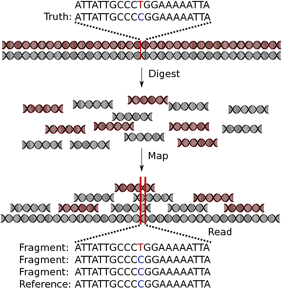
Here, this (diploid) individual has a SNP at the colored characters — one copy of a T and one of a C. What we eventually see is 1 T read and 2 C reads. From just these small read counts, we need to determine that the individual has 1 T allele and 1 C allele.
More realistically, we have dozens (or hundreds) of reads at each SNP (not just three). We can represent the inference problem in terms of a hexaploid species (having six copies of their genome) in the following “genotype plot”.
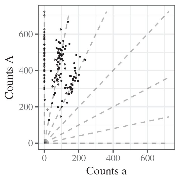
This scatterplot represents a single SNP. Each point is an individual. The x-axis is the number of “a” reads and the y-axis is the number “A” reads. The seven lines jutting out from (0,0) represent the expected counts at each of the seven possible genotypes for a hexaploid individual. The bottom right line is the expected counts for an individual with six copies of “a” (aaaaaa), the next line up is for individuals with five copies of “a” (Aaaaaa), then four copies (AAaaaa), etc.
Genotyping is equivalent to associating each point on this genotype plot with the line it belongs to. In the above plot, making this determination is relatively easy.
However, we found that making this determination can get really hard in a lot of other SNPs. Specifically, we had to deal with some issues present in GBS data: bias, overdispersion, and outlying points. But we worked at it and came up with a relatively good performing method to genotype individuals from GBS data — and it usually works a lot better than other methods out there because they do not account for these issues that we found.
The method is called updog for Using Parental Data for Offspring Genotyping. We named it this because we originally developed our approach when we had a sample of siblings, and so could wield this hierarchy to improve our genotyping. But the method works for general populations as well.
You can read more about updog in our preprint or our publication.
References
Gerard, D., Ferrão, L. F. V., Garcia, A. A. F., & Stephens, M. (2018). Genotyping Polyploids from Messy Sequencing Data. Genetics, 210(3), 789-807. doi:10.1534/genetics.118.301468 | bioRxiv:281550