Postdoctoral Work: Unobserved Confounding
The old work-horse of statistics is linear regression. It is an integral part of all scientific disciplines and genomics is no exception. Often, a biological scientist's goal will be to find associations between gene expression levels (how "active" a gene is) and a covariate of interest (such as whether or not a patient was given a drug, or whether or not a subject has a disease). To find these associations, biologists will often apply a simple linear regression model: \[ \boldsymbol{Y}_{n \times p} = \boldsymbol{X}_{n \times k}\boldsymbol{B}_{k \times p} + \boldsymbol{E}_{n \times p}, \] where \(y_{ij}\) is the gene expression level of gene \(j\) in sample \(i\), \(x_{ij}\) is the \(j\)th covariate for sample \(i\), the \(b_{ij}\)'s are the covariates of interest, and \(e_{ij}\) is some noise. This model works great if the modeling assumptions are correct. However, in most studies the true model is actually \[ \boldsymbol{Y}_{n \times p} = \boldsymbol{X}_{n \times k}\boldsymbol{B}_{k \times p} + \boldsymbol{Z}_{n \times q}\boldsymbol{A}_{q \times p} + \boldsymbol{E}_{n \times p}, \] where the columns of \(\boldsymbol{Z}\) are unobserved covariates, or confounders. Well-known examples include subject-level traits such as age/sex/ancestry, but also more innocent-sounding factors such as the lab or technician that processed a sample. Not accounting for unobserved confounding can have disasterous results on inference --- it can change the order of significance of genes and it can result in poor false discovery control.
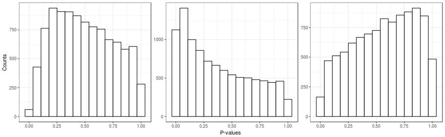
Unobserved confounding can be a problem even in the ideal case of a randomized experiment. Here's a simple example to illustrate this point. I took a real gene-expression dataset, \(\boldsymbol{Y}\), and I created a random covariate indicating group membership \(x_{i} \in \{0, 1\}\). I then calculated the simple two-sample \(t\)-tests for all of the genes (which is the same as fitting the naive model). Histograms for the \(p\)-values for three instances of the random covariate \(\boldsymbol{x}\) are presented in the figure below. Note that in these simulations, all genes are unnasociated with \(\boldsymbol{x}\), since the randomization was done independently of gene expression. Also recall that under the null hypothesis, \(p\)-values are distributed uniformly, and so we should see three flat histograms in the figure below. However, what we see in the figure are three very un-uniform-looking histograms. One way to understand this is to note that the same randomization is being applied to all genes. So if many genes are affected by an unobserved factor, and this factor happens by chance to be correlated with the randomization, then the \(p\)-value distributions will be non-uniform.
Unifying and Generalizing Confounder Adjustment Methods
The problem of unobserved confounding is known in the scientific community and there is an alphabet soup of methods that offer solutions: RUV2, RUV4, RUVinv, RUVrinv, RUVfun, CATEnc, scPLS, SSVA, LEAPP, CATErr, PEER, PANAMA, SVA, and others. All of these methods look similar on the surface, so one thing I wanted to do was understand how these methods are connected. I started by looking at the "RUV family" of methods above --- specifically RUV2 and RUV4.
One of the major difficulties in accounting for unobserved confounding is disentangling the effects of the observed covariates from the effects of the confounders correlated with the observed covariates. RUV2 and RUV4 use control genes (genes assumed to be unnassociated with the observed covariates) to make this determination, though they do so in different ways. RUV2 does factor analysis on the set of control genes to estimate the unobserved confounders then applies regression to estimate the effects of interest. RUV4 applies factor analysis on the residuals of a regression of \(\boldsymbol{X}\) on \(\boldsymbol{Y}\) and then disentangles the confounders from the observed covariates using the control genes.
Both of these methods requires an application of factor analysis, which in principal can be any form of factor analysis a user wants. So RUV2 and RUV4 are actually classes of methods indexed by the factor analyses used. I have shown that under certain conditions on the factor analyses, RUV2 and RUV4 are actually the exact same procedure.
This result is interesting for theoretical reasons, but it also hints at how to generalize RUV2 and RUV4. RUV2 only uses the control genes to estimate the confounders while RUV4 only uses the residuals to estimate the confounders. I developed RUV*, a general class of approaches that reframes confounder adjustment as a matrix-imputation problem. This allows two things: (1) the huge literature on matrix imputation may be weilded for confounder adjustment and (2) rather than just use the control genes or just use the residuals to estimate the confounders, we may develop methods to use both the control genes and the residuals to estimate the confounders. Under certain versions of RUV*, I have found that using all of the information possible to estimate the confounders and disentangle the effects of the covariates from those of the confounders results in more powerful and better calibrated procedures.
You can read more about this project in Gerard and Stephens (2021).
References
- Gerard, D., & Stephens, M. (2021). Unifying and Generalizing Methods for Removing Unwanted Variation Based on Negative Controls. Statistica Sinica 31(3), p. 1145–1166. doi:10.5705/ss.202018.0345 | arXiv:1705.08393