Environments
David Gerard
2022-02-15
Learning Objectives
- R Environments
- Chapter 7 from Advanced R
- These lecture notes are mostly taken straight out of Hadley’s book. Many thanks for making my life easier.
- His images, which I use here, are licensed under

Environment Basics
Hadley and colleagues made a really great package that, among other things, allows for handling environments:
{rlang}. It’s way better than the base R functionality.library(rlang)An environment is a fundamental data object in R that determines lexical scoping — i.e. they determine when a name is bound to an object.
Motivations:
- Environments are used to make functions self-contained.
- Environments are used to separate functions of the same name in different packages.
- Environments are used in some object oriented programming systems in R.
An environment is like a list, except:
- Every name must be unique.
- Lists can have multiple elements of the same name.
- Names are not ordered.
- Lists are ordered.
- All environments (except the empty environment) have “parent” environments that they live in.
- Environments use modify-in-place semantics.
- Lists are copy-on-modify.
- Every name must be unique.
Create a new environment with
rlang::env(), which behaves a lot listlist().e1 <- rlang::env(a = FALSE, b = "a", c = 2.3, d = 1:3)Environments associate names to values without any particular order. Hadley draws them like this:

Above, the arrows indicate “bindings”. So
bis bound to"a"andais bound toFALSE, etc…The blue dot indicates the parent environment.
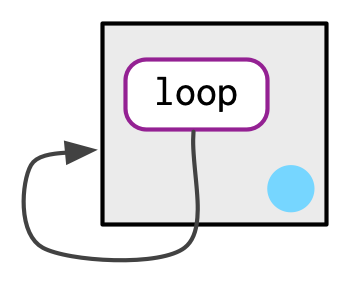
Environments have “reference semantics”, which means that they modify-in-place.
e2 <- e1
e2$d <- 4:6
e1$d
## [1] 4 5 6An environment can contain itself.
e1$d <- e1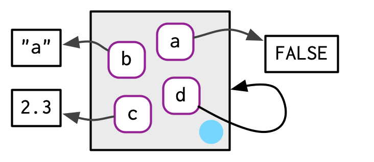
Printing an environment just shows its address in memory.
e1## <environment: 0x5594308c2588>To print the objects of an environment, use
rlang::env_print().rlang::env_print(e1)## <environment: 0x5594308c2588> ## Parent: <environment: global> ## Bindings: ## • a: <lgl> ## • b: <chr> ## • c: <dbl> ## • d: <env>Use
rlang::env_names()to get a character vector with names.rlang::env_names(e1)## [1] "a" "b" "c" "d"The current environment is the environment in which the code is currently being executed (where R looks for names). Use
rlang::current_env()to get the current environment.ce <- rlang::current_env() typeof(ce)## [1] "environment"The global environment is the environment where you interactively use R. You can access it with
rlang::global_env()gl <- rlang::global_env() typeof(gl)## [1] "environment"env_print(gl)## <environment: global> ## Parent: <environment: package:rlang> ## Bindings: ## • ce: <env> ## • e1: <env> ## • e2: <env> ## • gl: <env>We can see that the current environment is the global environment with
identical()identical(gl, ce)## [1] TRUEYou should not use
==. This is since==is expecting to be used on a vector, and an environment is not a vector.
Parents
Every environment has a parent. If a name is not found in the current environment then it is searched for in the parent. This is how lexical scoping operates in R.
rlang::env()actually creates a child environment. You can either supply the parent or it assumes the parent is the current environment.e2a <- env(d = 4, e = 5) e2b <- env(e2a, a = 1, b = 2, c = 3)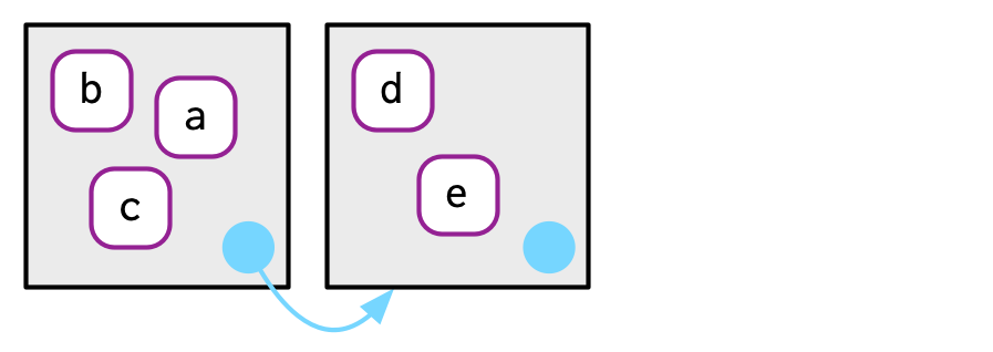
In the above diagram, the pale blue dot represents a pointer to the parent. The left box is the child and the right box is the parent.
rlang::env_parent()gives you the parent.env_parent(e2b)## <environment: 0x559433038710>e2a## <environment: 0x559433038710>env_parent(e2a)## <environment: R_GlobalEnv>Every environment has as an ancestor the empty environment, which has no parent. You can access it with
rlang::empty_env()em <- empty_env() rlang::env_print(em)## <environment: empty> ## Parent: NULLrlang::env_parents(em)## list()We can make children of the empty environment with
rlang::env()by including the empty environment as the first argument.e2c <- env(empty_env(), d = 4, e = 5) e2d <- env(e2c, a = 1, b = 2, c = 3)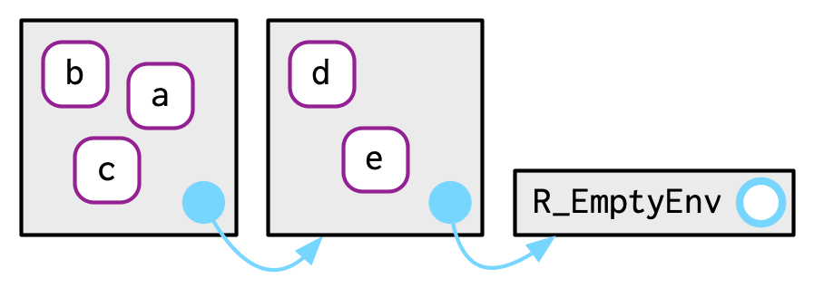
Your global environment has the empty environment as the progentor.
rlang::env_parents(rlang::global_env())## [[1]] $ <env: package:rlang> ## [[2]] $ <env: package:stats> ## [[3]] $ <env: package:graphics> ## [[4]] $ <env: package:grDevices> ## [[5]] $ <env: package:utils> ## [[6]] $ <env: package:datasets> ## [[7]] $ <env: package:methods> ## [[8]] $ <env: Autoloads> ## [[9]] $ <env: package:base> ## [[10]] $ <env: empty>The ancestors of the global environment are all of the attached packages that ultimately terminate in the empty environment. So
env_parents()will stop at the global environment by default.et <- rlang::env(x = 1:3) rlang::env_parents(et)## [[1]] $ <env: global>rlang::env_parents(et, last = rlang::empty_env())## [[1]] $ <env: global> ## [[2]] $ <env: package:rlang> ## [[3]] $ <env: package:stats> ## [[4]] $ <env: package:graphics> ## [[5]] $ <env: package:grDevices> ## [[6]] $ <env: package:utils> ## [[7]] $ <env: package:datasets> ## [[8]] $ <env: package:methods> ## [[9]] $ <env: Autoloads> ## [[10]] $ <env: package:base> ## [[11]] $ <env: empty>
Working with Objects in an Environment
Regular assignment
<-creates a variable in the current environment.Super assignment
<<-modifies an existing variable found in the parent environment. If no such variable exists, it creates one in the global environment.x <- 0 f <- function() { x <<- 1 } f() x## [1] 1Most of the time, it is not a good idea to use super assignment. Global variables are vary dangerous. We’ll talk about one good application of them in Chapter 10.
Get and set values from an environment the same way as from a list.
e3 <- env(x = 1, y = 2)
e3$x
## [1] 1e3[["x"]]## [1] 1Because environments are unordered, integer subsetting does not work
e3[[1]]## Error in e3[[1]]: wrong arguments for subsetting an environmentBecause environments are not vectors, you cannot use sing brackets
[], so you cannot get more than one element.e3["x"]## Error in e3["x"]: object of type 'environment' is not subsettablee3[c("x", "y")]## Error in e3[c("x", "y")]: object of type 'environment' is not subsettableYou get
NULLif a variable is not in an environment, just like a list:e3$z## NULLTest if an environment has a binding with
rlang::env_has()rlang::env_has(e3, "x")## x ## TRUErlang::env_has(e3, "z")## z ## FALSEUnlike a list, you do not remove elements by assigning them to
NULL, because the name refers toNULL.e3$a <- 10 e3$a <- NULL e3$a## NULLrlang::env_has(e3, "a")## a ## TRUEUse
rlang::env_unbind()to remove an object.rlang::env_unbind(e3, "a") rlang::env_has(e3, "a")## a ## FALSE
Hadley’s Advanced R Exercises
Create an environment as illustrated by this picture.
Create a pair of environments as illustrated by this picture.
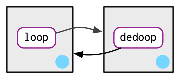
Loop through environments
Sometimes, you want to look through all of the ancestor environments to find an object, or for exploration. Here is an example where we count how many objects are in each ancestral environment.
count_env <- function(base_env = rlang::caller_env(),
                      end_env = rlang::empty_env()) {
  nenv <- length(rlang::env_parents(env = base_env, last = end_env))
  obj_num <- rep(NA_real_, length.out = nenv)
  env <- base_env
  for(i in seq_len(nenv)) {
    obj_num[[i]] <- length(env)
    names(obj_num)[[i]] <- rlang::env_name(env)
    env <- rlang::env_parent(env)
  }
  return(obj_num)
}
count_env()
## global package:rlang package:stats package:graphics ## 14 434 456 88 ## package:grDevices package:utils package:datasets package:methods ## 119 221 104 371 ## Autoloads package:base ## 1 1370The caller environment is the environment of the function that called the current function. See below.
Special Environments
Most environments are created by R, not by you.
The most important ones are:
Global Environment: Environment that you, the user, interact with during an interactive session.
Package Environment: External interface for a package. When you, the user, uses a function, it looks for it in the package environment.
Namespace Environment: Internal interface for apackage. When the package searches for a function within the same package, it looks for it in the namespace environment.
Imports Environment: Functions used by the package. When the package searches for a function from another package, it looks for it in the imports environment.
Function Environment (aka enclosing environment): Environment where function was created and where it has access to objects. For a function from a package, this is the namespace environment. For a function you create during an interactive session, this is the global environment.
Binding Environment of a function: Environment where the name of a function is bound to the function. May or may not be the same as the function environment.
Execution Environment: Each time a function is called, a new temporary environment is created to host execution. This is to that function calls always have a “fresh start”
Caller environment: The environment in which the function was called.
Package environments.
Each package attached by
library()creates a package environment that becomes an ancestor of the global environment. They are parents in the order that you attached them.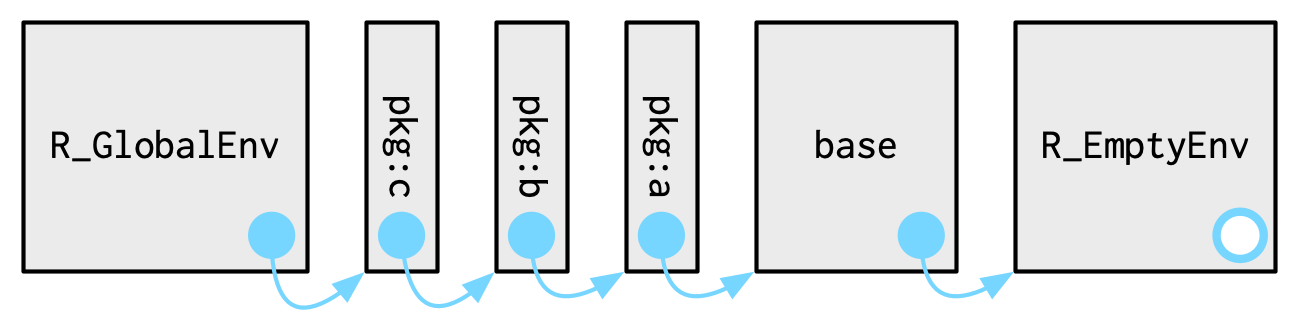
This order is called the search path because variable names are searched in that order. You can see the search path with
rlang::search_envs().rlang::search_envs()## [[1]] $ <env: global> ## [[2]] $ <env: package:rlang> ## [[3]] $ <env: package:stats> ## [[4]] $ <env: package:graphics> ## [[5]] $ <env: package:grDevices> ## [[6]] $ <env: package:utils> ## [[7]] $ <env: package:datasets> ## [[8]] $ <env: package:methods> ## [[9]] $ <env: Autoloads> ## [[10]] $ <env: package:base>So if I try to evaluate a variable/function name, then it will first search for it in the global environment, then in the
{rlang}package environment, then in the{stats}package environment, etc…Attaching a new package with
library()makes that package the immediate parent of the global environment.library(d)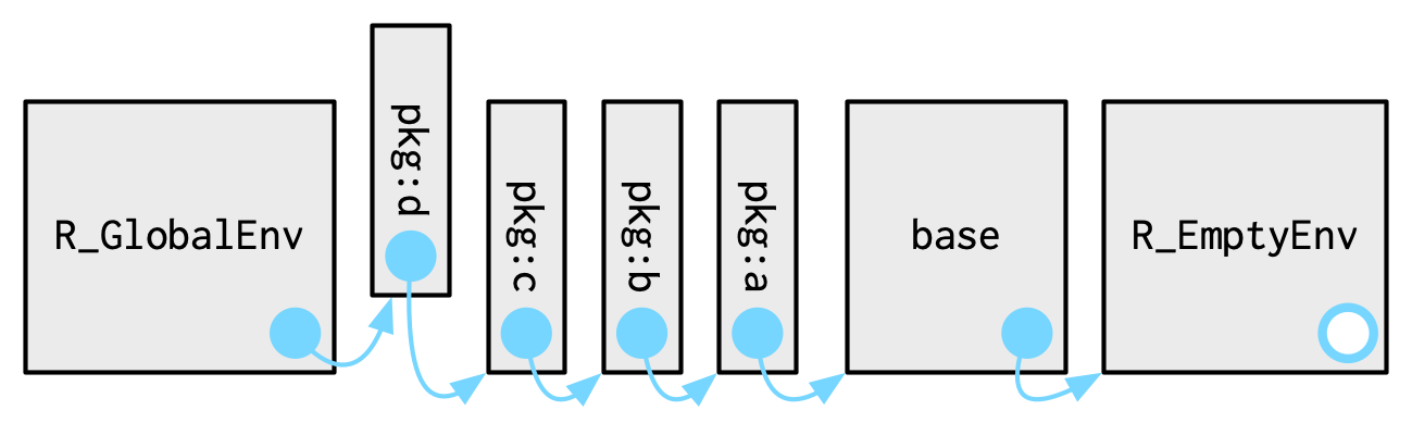
Function Environment
The function environment is the environment where the function has access to all objects in that environment and its parent environments. This is the current environment when the function is created, not when the function is called.
You can see the function environment via
rlang::fn_env()The function environment may or may not be a new environment. E.g. most of the functions you write use the global environment as the function environment.
x <- 5
fn <- function() {
  sum(1:x)
}
rlang::fn_env(fn)
## <environment: R_GlobalEnv>Above, since the function environment is the global environment,
fn()has access tox(which is in the global environment) and tosum()(which is in the namespace:base environment).Most functions in a package have the namespace environment (see below) as the function environment.
rlang::fn_env(base::sum)## <environment: namespace:base>rlang::fn_env(stats::lm)## <environment: namespace:stats>rlang::fn_env(rlang::fn_env)## <environment: namespace:rlang>The function environment may or may not be different from the environment where the name is bound to the function. That space is called the binding environment of the function.
In many cases, the function environment is the same as the binding environment. Below, the name
fin the global environment is bound to the function (arrow moving from f to the yellow object), so the binding environment is the global environment. Also below, the function is bound to the global environment (arrow moving from the black dot to the global environment), so the global environment has the objects that the function has access to, so the function environment is also the global environment.y <- 1 f <- function(x) { return(x) }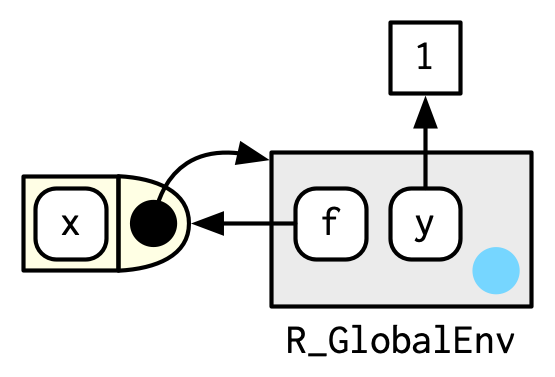
Below, the name
gin theeenvironment was created in the global environment. So the function environment is the global environment. But the namegis in theeenvironment, so the binding environment ise.y <- 1 e <- rlang::env() e$g <- function(x) { return(x) }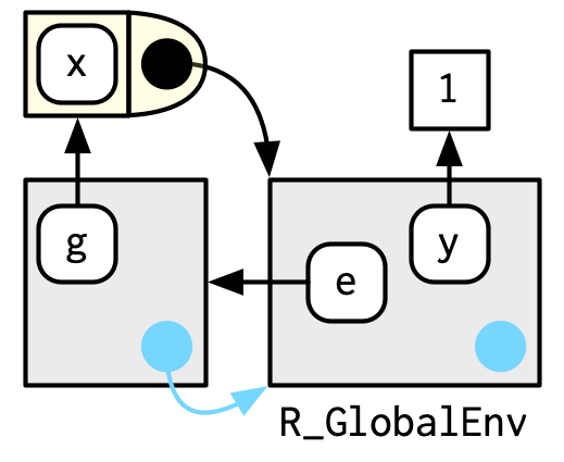
Exercise: Does
g()still have access to all of the objects in the global environment?
Namespaces
The package environment is the external interface for a package. It contains the exported functions of a package.
The namespace environment of a package is the internal interface for a package. Functions in the package will search for its objects in the namespace environment.
This is what allows us to modify (rather foolishly)
var()but still allowsd()to work properly.sd## function (x, na.rm = FALSE) ## sqrt(var(if (is.vector(x) || is.factor(x)) x else as.double(x), ## na.rm = na.rm)) ## <bytecode: 0x55943244bc68> ## <environment: namespace:stats>x <- rnorm(10) sd(x)## [1] 0.6674var <- function(x) 0 var(x)## [1] 0sd(x)## [1] 0.6674The namespace environment acts as the function environment for all functions in a package.
An exported function has a binding both in the namespace environment and the package environment.
An internal function only has a binding the namespace environment.
The parent of a namespace environment is an imports environment that contains bindings of all functions used by the package.
The parent of the imports environment is the base namespace, where all base functions are located (this is why you don’t need to import
sum()or usebase::sum()in your package code).The parent of the base namespace is the global environment.
library(rlang)
env_parents(fn_env(stats::var))
## [[1]] $ <env: imports:stats> ## [[2]] $ <env: namespace:base> ## [[3]] $ <env: global>env_parents(fn_env(rlang::fn_env))## [[1]] $ <env: imports:rlang> ## [[2]] $ <env: namespace:base> ## [[3]] $ <env: global>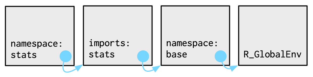
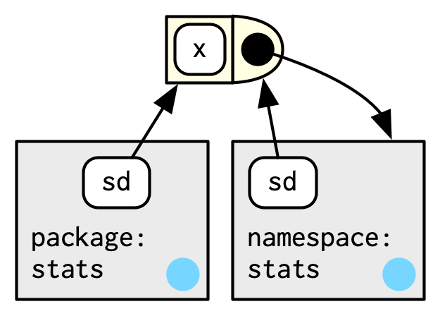
Below, let the yellow object be the
sd()function defined in the package{stats}. Then whenever another function in{stats}usessd()orvar()it finds them in thenamespace:statsenvironment. Right now, thepackage:statsenvironment also points to that function, so when the user usessd()they can use the version created by the{stats}authors. However, if we change the definition ofvar(), we only change the binding in thepackage:statsenvironment, not in thenamespace:statsenvironment. This means that{stats}functions will work even if we change the binding. In particular,sd(), which usesvar(), will still work.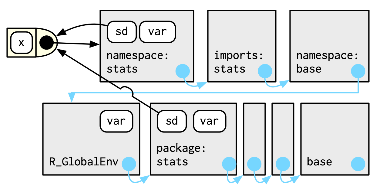
Execution Environments
Each time a function is called, a new environment is created to host execution. This is called the execution environment.
This is why
ais not saved between calls:fn <- function() { if (!env_has(current_env(), "a")) { a <- 1 } else { a <- a + 1 } return(a) } fn()## [1] 1fn()## [1] 1The execution environment is always the child of the function environment.
Consider this function
h <- function(x) {
  # 1.
  a <- 2 # 2.
  x + a
}
y <- h(1) # 3.
The yellow object is the
h()function. The namehis in the global environment (bottom right). The execution environment is the top left.xbinds to 1. Thenais defined, it binds to2. When the function completes, it returns3and soybinds to3in the global environment. The execution environment is garbage collected.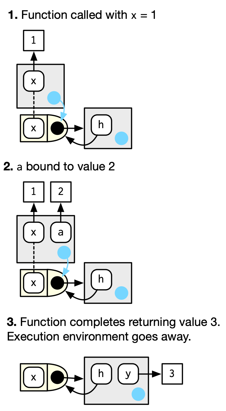
It is possible to explicitly return the execution environment so that it is not garbage collected. But this is rarely done.
h2 <- function(x) {
  a <- x * 2
  rlang::current_env()
}
e <- h2(x = 10)
rlang::env_print(e)
## <environment: 0x559433fd0850> ## Parent: <environment: global> ## Bindings: ## • a: <dbl> ## • x: <dbl>More frequently, the execution environment is maintained because it is a function environment of a returned function.
plus <- function(x) {
  function(y) x + y
}

plus_one <- plus(1)
plus_one
## function(y) x + y ## <environment: 0x559430a38cc8>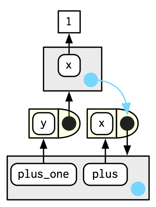
Above figure: the global environment is the bottom box. The execution environment is the top box. The
plus()function is the right yellow object. Its function environment and binding environment is the global environment. Whenplus()is called withx = 1, it creates the execution environment wherexis bound to1. Whenplus_one()is defined, its function environment is the execution environment (since that is where it was created), but its binding environment is the global environment (where the name is bound). Note that the parent environment of theplus()’s execution environment is the global environment.rlang::fn_env(plus_one)## <environment: 0x559430a38cc8>rlang::env_parent(rlang::fn_env(plus_one))## <environment: R_GlobalEnv>When we call
plus_one(), its execution environment will have the execution environment ofplus()as its parent.x <- 20 plus_one(2)## [1] 3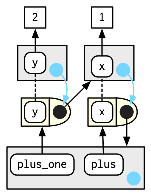
When we call
plus_one()withybound to 2 (execution environment top left), when it tries to findxit first searches inrlang::fn_env(plus_one)## <environment: 0x559430a38cc8>(execution environment top right) before going to the global environment (bottom).
Exercise (Advanced R): Draw a diagram that shows the function environments of this function, along with all bindings for the given execution.
f1 <- function(x1) {
  f2 <- function(x2) {
    f3 <- function(x3) {
      x1 + x2 + x3
    }
    f3(3)
  }
  f2(2)
}
f1(1)
## [1] 6
Caller Environment
Recall, the function environment is the environment in which the function was created.
The caller environment is the environment in which the function was called (aka “used”)
You can get this environment inside a function via
rlang::caller_env().fn1 <- function(x) { fn2 <- function(y) { rlang::caller_env() } e0 <- rlang::current_env() ## The execution environment of fn1() e1 <- fn2() ## The caller environment of fn2() e2 <- rlang::caller_env() ## The caller environment of fn1() return(list(e0, e1, e2)) } fn1()## [[1]] ## <environment: 0x559432c478c8> ## ## [[2]] ## <environment: 0x559432c478c8> ## ## [[3]] ## <environment: R_GlobalEnv>
Applications
Numeric Derivatives
stats::numericDeriv()numerically evaluates the gradient of an expression at some value. It assumes that the evaluation occurs within some environment you provide.Let’s calculate the gradient of \(x^y\) evaluated at \(x = 3\).
myenv <- rlang::env(x = 3, y = 2)
numericDeriv(expr = rlang::expr(x ^ y), theta = "x", rho = myenv)
## [1] 9 ## attr(,"gradient") ## [,1] ## [1,] 6From calculus, we know that the derivative of \(x^2\) is \(2x\), and so the gradient evaluated at \(x = 3\) should be \(2\times 3 = 6\).
rlang::expr()is discussed in Chapter 19. Basically, it captures an expression without evaluating it. This is called “quoting”. We can then evaluate that expression witheval().rlang::expr(x^2)## x^2rlang::expr(x^2) |> eval(envir = myenv)## [1] 9rlang::expr(sum(c(1, 2, 3)))## sum(c(1, 2, 3))rlang::expr(sum(c(1, 2, 3))) |> eval(envir = rlang::global_env())## [1] 6
Managing State
An R package cannot alter the global environment.
Objects in packages are locked, so cannot be changed.
Say you want to keep track of whether or not a function was run (e.g. to write a message on first use). I have done this to (i) say that a function is defunct or (ii) list out special licenses that cover a method.
One way you could keep track of this is to use super assign in a function that will change the value of a logical in the package environment.
ran_fun <- FALSE ## Global variable
fun <- function() {
  if (!ran_fun) {
    message("Here is a message")
    ran_fun <<- FALSE ## this alters package environment
  }
}
fun()
## Here is a messagefun()## Here is a messageWhat I think is better is having an environment specific to messages, that way you have to worry less about global variables.
menv <- rlang::env(ran_fun = FALSE)
fun <- function() {
  if (!menv$ran_fun) {
    message("Here is a message")
    menv$ran_fun <- TRUE
  }
}
fun()
## Here is a messagefun()This functionality is very popular, so
{rlang}has a function dedicated to it.fun <- function() { rlang::warn("Here is a message", .frequency = "once", .frequency_id = "ran_fun") } fun()## Warning: Here is a message ## This warning is displayed once per session.fun()Exercise: Use environments to keep a tally for how many times a function called
foo()is run. Create another function calledfoo_count()that returns that number. E.g.foo_count()## [1] 0foo() foo() foo() foo_count()## [1] 3
R6 Objects
- We will not cover R6 objects, but they use environments to do modify-by-reference instead of copy-on-modify semantics. This makes them fast.
Hashing
Hashing is a quick way to select an object from a bunch of possible objects. You use a hash key to select a hash value.
Hashing in R was done through the
{hash}package using environments.Hashing is way quicker than using a list or a vector.
In the below example, using hashing is about 1000 times faster than using native R vectors.
library(hash)
words <- read.table("https://data-science-master.github.io/lectures/data/words.txt",
                    header = TRUE,
                    na.strings = "")
h <- hash(keys = words$word, values = seq_along(words$word))
l <- seq_along(words$word)
names(l) <- words$word

bench::mark(
  h$MOTIVITIES,
  l[["MOTIVITIES"]],
) |>
  dplyr::select(expression:result) |>
  knitr::kable()
expression min median itr/sec mem_alloc gc/sec n_itr n_gc total_time result h$MOTIVITIES 1.4µs 1.48µs 460833.6 0B 0 10000 0 21.7ms 150000 l[[“MOTIVITIES”]] 1.69ms 1.79ms 543.9 0B 0 272 0 500.1ms 150000 Though, for this lookup to be worthwhile, you would need to be doing lookups millions of times a second.
New Functions
rlang::env(): Create a new child environment.rlang::env_print(): Print an environment’s bindings.rlang::env_names(): Print names in an environment.rlang::env_parent(): Print the parent of an environment.rlang::env_has(): Test if an environment has a binding.rlang::current_env(): Access current environment.rlang::env_bind(): Add objects to an environment.rlang::env_unbind(): Remove objects from an environment.rlang::global_env(): Access global environment.rlang::empty_env(): Access the empty environment.rlang::fn_env(): Access the function environment.rlang::caller_env(): Access the caller environment.rlang::search_envs(): Show the search path.identical(): Check if two objects are exactly equal.

This work is licensed under a Creative Commons Attribution-NonCommercial 4.0 International License.