Learning Objectives

Required Reading:
More resources:

Motivation

The most common application of S4 objects is in the Bioconductor project, so we will use some of the classes from that project as an example.
Bioconductor also provides some of the best software to analyze genomic data. Being able to use it is vital for genomic researchers.
Bioconductor is huge, and learning that ecosystem would take a semester. Here, we will just learn the basic data types used within the {VariantAnnotation} package.

Bioconductor Setup

Bioconductor is a repository for hosting R packages (just like CRAN).
But Bioconductor packages are focused on biological applications. They also share S4 objects between packages that are designed to make analyzing biological data easier.
You do not use install.packages() to install packages from Bioconductor, you use BiocManager::install(). So first make sure you have {BiocManager} installed on your computer:
```
install.packages("BiocManager")
```
Now install the {VariantAnnotation} package, which is used for storing and manipulating genomic variants.
```
BiocManager::install("VariantAnnotation")
```
One thing you will notice from Bioconductor is that all S4 classes and most packages are in UpperCamelCase, and S4 methods are in lowerCamelCase.
For anything Bioconductor related, you can get help by searching the support site: https://support.bioconductor.org/

Basic Objects

The {VariantAnnotation} package uses a lot of S4 objects which are common in the Bioconductor ecosystem.
```
library(VariantAnnotation)
```
We will go through these classes before discussing the {VariantAnnotation} package itself.

`SimpleList`

The SimpleList class is the S4 version of the basetype list.
The SimpleList is defined in the {S4Vectors} package.

Wherever you used a list, you can also use a SimpleList.

sval <- SimpleList(a = 1:4,
                   b = c("A", "B", "C"))
sloop::otype(sval)

## [1] "S4"

class(sval)

## [1] "SimpleList"
## attr(,"package")
## [1] "S4Vectors"

sval

## List of length 2
## names(2): a b

sval$a

## [1] 1 2 3 4

sval$b

## [1] "A" "B" "C"

Internally (i.e. hidden from the user), the slots are
- @listData: A list containing the data.
- @elementType: A character of length 1 describing the subclass of the SimpleList.
- @elementMetadata: Annotates individual elements of the SimpleList.
- @metadata: Annotates the SimpleList as a whole.

`DataFrame`

The DataFrame is an S4 version of a data.frame (which is an S3 class).
The DataFrame class is from the {S4Vectors} package.

Most of the operations you are used to for data.frames can be used for DataFrames.

df <- DataFrame(a = 1:3,
                b = c("A", "B", "C"))
sloop::otype(df)

## [1] "S4"

df

## DataFrame with 3 rows and 2 columns
##           a           b
##   <integer> <character>
## 1         1           A
## 2         2           B
## 3         3           C

df$a

## [1] 1 2 3

df[, 2]

## [1] "A" "B" "C"

Two differences:

The row.names attribute is optional in DataFrames, but is required in data.frames.
The DataFrame object can have an slot called elementMetadata, which is a another DataFrame where each row indexes one of the columns of the original DataFrame. So each row of the metadata contains information on each column of the data. You set and get this metadata with mcols().

row.names(df) ## no row.names

## NULL

mcols(df) <- DataFrame(DataFrame(info = c("1st", "2nd"),
                                 description = c("random", "stuff")))
mcols(df)

## DataFrame with 2 rows and 2 columns
##          info description
##   <character> <character>
## a         1st      random
## b         2nd       stuff

There are other methods for DataFrame objects that do not exist for data.frame objects. See
```
?`DataFrame-class`
?`DataFrame-combine`
?`DataFrame-utils`
```

`CharacterList`, `NumericList`, `IntegerList`, `LogicalList`

These atomic lists are extensions of the S4 List object that only holds atomic vectors.
These are defined in the {IRanges} package.

E.g. an IntegerList can have many elements, but each one has to be an integer vector.

il <- IntegerList(a = c(1L, 2L, 3L),
                  b = c(4L, 5L, 6L, 7L, 8L))
il

## IntegerList of length 2
## [["a"]] 1 2 3
## [["b"]] 4 5 6 7 8

The reason to define lists in this way, is that you can perform operations simultaneously on all vectors in these atomic lists.

il + 1L

## IntegerList of length 2
## [["a"]] 2 3 4
## [["b"]] 5 6 7 8 9

il == 2

## LogicalList of length 2
## [["a"]] FALSE TRUE FALSE
## [["b"]] FALSE FALSE FALSE FALSE FALSE

max(il)

## a b 
## 3 8

sum(il)

##  a  b 
##  6 30

See the following for more information
```
?`AtomicList`
?`AtomicList-utils`
```

`Rle`

The Rle class is a an atomic vector that can more efficiently store vectors with long repeats via run-length encoding.
It is defined in the {S4Vectors} package.
Instead of storing the entire vector when there are lots of repeats, run-length encoding just stores the values that are repeated (“values”) along with the number of times they are repeated (“lengths”).

Consider this vector with lots of repeats

x <- rep(c("A", "C", "T", "G"), 1:4)
x

##  [1] "A" "C" "C" "T" "T" "T" "G" "G" "G" "G"

We can instead store it as

“A” is copied once.
“C” is copied twice.
“T” is copied three times.
“G” is copied four times.

base::rle(x)

## Run Length Encoding
##   lengths: int [1:4] 1 2 3 4
##   values : chr [1:4] "A" "C" "T" "G"

The Rle class does this run-length encoding behind-the-scenes.

Let’s generate some very long data with lots of repeats:

lambda <- c(rep(0.001, 4500), 
            seq(0.001, 10, length=500), 
            seq(10, 0.001, length=500))
pvec <- rpois(1e6, lambda)
head(pvec)

## [1] 0 0 0 0 0 0

rvec <- Rle(pvec)

The size of the objects is dramatically different.

lobstr::obj_size(pvec)

## 4,000,048 B

lobstr::obj_size(rvec)

## 1,204,040 B

You can treat Rle objects just like regular vectors.

rvec[100]

## integer-Rle of length 1 with 1 run
##   Lengths: 1
##   Values : 0

rvec + 1

## numeric-Rle of length 1000000 with 150359 runs
##   Lengths: 1765    1  307    1 2114    1  113 ...    1 1701    1  332    1 1003
##   Values :    1    2    1    2    1    2    1 ...    2    1    2    1    2    1

length(rvec)

## [1] 1000000

sum(rvec)

## [1] 905333

Rle has more efficient ways to subset regions via the window() generic.

window(rvec, 510445, 788990)

## integer-Rle of length 278546 with 42354 runs
##   Lengths:   67    1    1    1    3    2    2 ...    4    2    1 1218    1 1273
##   Values :    0    1    0    1    0    1    0 ...    1    0    1    0    1    0

Get the run lengths via runLength()

head(runLength(rvec))

## [1] 1765    1  307    1 2114    1

Get the values via runValue()
```
head(runValue(rvec))
```
```
## [1] 0 1 0 1 0 1
```
This class is really beneficial for genomic data, where DNA often has sequences of long repeats.
See the following for more operations available on Rle objects.
```
?`Rle-class`
?`Rle-utils`
?`Rle-runstat`
```

`IRanges`

The IRanges class contains two integer vectors. The first specifies “start” positions, the second specifies “width” of the position.
You should consider an IRanges object like a vector, where each element has a start position and a width.

The idea is that you might want to describe what part of the genome you are considering (e.g. from base pair 107889 of width 2000 base pairs) without having to describe the sequence in that range.

iobj <- IRanges(start = c(5, 1001, 59999), width = c(87, 70, 101))
iobj

## IRanges object with 3 ranges and 0 metadata columns:
##           start       end     width
##       <integer> <integer> <integer>
##   [1]         5        91        87
##   [2]      1001      1070        70
##   [3]     59999     60099       101

The “end” positions is not an internal slot. It is just printed via the show() method of the IRanges class.

You can access the start, end, and widths of the ranges via

start(iobj)

## [1]     5  1001 59999

end(iobj)

## [1]    91  1070 60099

width(iobj)

## [1]  87  70 101

You can subset like a regular vector

iobj[1]

## IRanges object with 1 range and 0 metadata columns:
##           start       end     width
##       <integer> <integer> <integer>
##   [1]         5        91        87

You can choose to only include regions that begin or end at some position

iobj[start(iobj) > 100]

## IRanges object with 2 ranges and 0 metadata columns:
##           start       end     width
##       <integer> <integer> <integer>
##   [1]      1001      1070        70
##   [2]     59999     60099       101

I ranges are often used to extract elements with regions of interest.

E.g., remember the Rle object that we constructed:

rvec

## integer-Rle of length 1000000 with 150359 runs
##   Lengths: 1765    1  307    1 2114    1  113 ...    1 1701    1  332    1 1003
##   Values :    0    1    0    1    0    1    0 ...    1    0    1    0    1    0

What if we want to get the values within the ranges that we constructed via the IRanges object? Then we just use regular bracket subsetting:

rvec[iobj]

## integer-Rle of length 258 with 95 runs
##   Lengths: 157   1   1   1   1   1   1   1 ...   1   1   1   1   1   1   1   1
##   Values :   0   6  15  11   7  12  13  14 ...   4  12   8  11   5   6   9   4

There is lots more that IRanges implements. See the help file for more.
```
?`IRanges-class`
```

`GRanges`

The GRanges S4 class is a vector-like class that represents genomic locations and their annotations.
This class is defined in the {GenomicRanges} package.
Each element of a GRanges class contains (i) a sequence name, (ii) an interval of the sequence’s location, (iii) the strand, (iv) optional sequence information, and (v) some optional metadata.
Below are the slots:
- @seqnames: An Rle object containing the sequence names (like chromosome 1, or mitochondrial chromosome, etc…). Multiple elements can have the same sequence name (e.g. many parts of the genome belong to chromosome 1).
- @ranges: An IRanges object containing the location and ranges of the DNA sequence.
- @strand: An RLE object containing the strand information.
- @seqinfo: Optionally provided. This is a Seqinfo class object (which we haven’t covered) which contains metainformation on each sequence name. Specifically, the sequence name, the sequence length, whether the chromosome is circular, and the genome that the sequence comes from (like a specific assembly of the human genome)
- @elementMetadata: An optional DataFrame object containing metainformation for each element. The rows index the different locations on the genome and the columns index different types of metainformation.
Extreme Biology Note: Recall that DNA is a double helix with “A” paired with “T” and “G” paired with “C.” So you can read the sequences going in one direction (ATTTG) or in the other direction (CAAAT). One direction, which is the same order in which RNA builds proteins, is called the “sense” strand, or the “+” strand, or the 5’ to 3’ strand. The other direction, which is not the same direction that RNA uses to build proteins, is called the “antisense” strand, or the “-” strand, or the 3’ to 5’ strand. In Bioconductor, they use notations “+,” “-,” and “*” for when the strand is undetermined (or does not matter).
```
gr1 <- GRanges(seqnames = Rle(c("ch1", "chMT"), c(2, 4)),
               ranges = IRanges(16:21, 20),
               strand = rep(c("+", "-", "*"), 2))
gr1
```
```
## GRanges object with 6 ranges and 0 metadata columns:
##       seqnames    ranges strand
##          <Rle> <IRanges>  <Rle>
##   [1]      ch1     16-20      +
##   [2]      ch1     17-20      -
##   [3]     chMT     18-20      *
##   [4]     chMT     19-20      +
##   [5]     chMT        20      -
##   [6]     chMT     21-20      *
##   -------
##   seqinfo: 2 sequences from an unspecified genome; no seqlengths
```

These are the various getters for the slots:

seqnames(gr1)

## factor-Rle of length 6 with 2 runs
##   Lengths:    2    4
##   Values : ch1  chMT
## Levels(2): ch1 chMT

ranges(gr1)

## IRanges object with 6 ranges and 0 metadata columns:
##           start       end     width
##       <integer> <integer> <integer>
##   [1]        16        20         5
##   [2]        17        20         4
##   [3]        18        20         3
##   [4]        19        20         2
##   [5]        20        20         1
##   [6]        21        20         0

strand(gr1)

## factor-Rle of length 6 with 6 runs
##   Lengths: 1 1 1 1 1 1
##   Values : + - * + - *
## Levels(3): + - *

seqinfo(gr1)

## Seqinfo object with 2 sequences from an unspecified genome; no seqlengths:
##   seqnames seqlengths isCircular genome
##   ch1              NA         NA   <NA>
##   chMT             NA         NA   <NA>

mcols(gr1)

## DataFrame with 6 rows and 0 columns

You can access start, end, and width directions directly without first extracting the @ranges slot.
```
start(gr1)
```
```
## [1] 16 17 18 19 20 21
```
```
end(gr1)
```
```
## [1] 20 20 20 20 20 20
```
```
width(gr1)
```
```
## [1] 5 4 3 2 1 0
```

You should think of a GRanges object as a vector where each element is a location on the genome.

gr1[1]

## GRanges object with 1 range and 0 metadata columns:
##       seqnames    ranges strand
##          <Rle> <IRanges>  <Rle>
##   [1]      ch1     16-20      +
##   -------
##   seqinfo: 2 sequences from an unspecified genome; no seqlengths

length(gr1)

## [1] 6

gr1[start(gr1) > 18]

## GRanges object with 3 ranges and 0 metadata columns:
##       seqnames    ranges strand
##          <Rle> <IRanges>  <Rle>
##   [1]     chMT     19-20      +
##   [2]     chMT        20      -
##   [3]     chMT     21-20      *
##   -------
##   seqinfo: 2 sequences from an unspecified genome; no seqlengths

See more by
```
?`GRanges-class`
```

`DNAString`

The DNAString class (from the {Biostrings} package) allows for efficient storage of a single DNA sequence.
The idea is that a DNAString is a single short sequence, or a whole chromosome, but only one contiguous sequence.
```
dna1 <- DNAString("ACGT-N")
dna1
```
```
## 6-letter DNAString object
## seq: ACGT-N
```
This is the same as a character except it can only be length 1, and there is a limit to the types of characters possible.

The different characters possible are found via

IUPAC_CODE_MAP

##      A      C      G      T      M      R      W      S      Y      K      V 
##    "A"    "C"    "G"    "T"   "AC"   "AG"   "AT"   "CG"   "CT"   "GT"  "ACG" 
##      H      D      B      N 
##  "ACT"  "AGT"  "CGT" "ACGT"

E.g. “B” means that the nucleotide could be C, G, or T, but not A.

In addition, “-” means a gap (because of an alignment comparing sequences, not an actual physical gap).
Sequence length is found by length() or ncar() methods.
```
length(dna1)
```
```
## [1] 6
```
```
nchar(dna1)
```
```
## [1] 6
```
You can access a subsequence by bracket subsetting
```
dna1[2:4]
```
```
## 3-letter DNAString object
## seq: CGT
```
See more by
```
?`DNAString-class`
```

`DNAStringSet`

The DNAStringSet is a like a character vector, except each element is a DNAString instead of a string.

This class is also from the {Biostrings} package.

ds <- DNAStringSet(x = c("AAAGCC", "ACTATC", "TGCNNAA-CCTT"))
ds

## DNAStringSet object of length 3:
##     width seq
## [1]     6 AAAGCC
## [2]     6 ACTATC
## [3]    12 TGCNNAA-CCTT

It operates like a character vector

ds[[1]]

## 6-letter DNAString object
## seq: AAAGCC

ds[1:2]

## DNAStringSet object of length 2:
##     width seq
## [1]     6 AAAGCC
## [2]     6 ACTATC

length(ds)

## [1] 3

You can operate on all DNA sequences at the same time with a few operations. E.g.

subseq(ds, start = 2, end = 4)

## DNAStringSet object of length 3:
##     width seq
## [1]     3 AAG
## [2]     3 CTA
## [3]     3 GCN

See more by
```
?`DNAStringSet-class`
```

`DNAStringSetList`

The DNAStringSetList class (also from {Biostrings}) is a list-like class where each element is a DNAStringSet.

dna1 <- c("AAA", "AC", "", "T", "GGATA")
dna2 <- c("G", "TT", "C")
x <- DNAStringSetList(dna1, dna2)
x

## DNAStringSetList of length 2
## [[1]] AAA AC  T GGATA
## [[2]] G TT C

This is useful for storing multiple possible alleles that are varying in the population. E.g. below indicates that the first location is an A, the second is either an A or G, and the third is either an A or a T or a G.
```
dna_ex <- DNAStringSetList("A", c("A", "G"), c("A", "T", "G"))
dna_ex
```
```
## DNAStringSetList of length 3
## [[1]] A
## [[2]] A G
## [[3]] A T G
```
See more by
```
?`DNAStringSetList-class`
```

Basic Data Exercises

Create a DNAStringSet object of length 100 that contains just A’s. That is

## DNAStringSet object of length 100:
##       width seq
##   [1]     1 A
##   [2]     1 A
##   [3]     1 A
##   [4]     1 A
##   [5]     1 A
##   ...   ... ...
##  [96]     1 A
##  [97]     1 A
##  [98]     1 A
##  [99]     1 A
## [100]     1 A

Create a DNAStringSetList object of length 100 that contains just c(C, G)’s. That is:

## DNAStringSetList of length 100
## [[1]] C G
## [[2]] C G
## [[3]] C G
## [[4]] C G
## [[5]] C G
## [[6]] C G
## [[7]] C G
## [[8]] C G
## [[9]] C G
## [[10]] C G
## ...
## <90 more elements>

Create an IRanges object of where the start positions are 100, 200, …, 10000, and the widths are 1, 2, 3, …, 100. That is,

## IRanges object with 100 ranges and 0 metadata columns:
##             start       end     width
##         <integer> <integer> <integer>
##     [1]       100       100         1
##     [2]       200       201         2
##     [3]       300       302         3
##     [4]       400       403         4
##     [5]       500       504         5
##     ...       ...       ...       ...
##    [96]      9600      9695        96
##    [97]      9700      9796        97
##    [98]      9800      9897        98
##    [99]      9900      9998        99
##   [100]     10000     10099       100

Create a GRanges object using your results from exercise 3 where the seqname is "chr1" for all loci, and the strand is "*" for all loci. That is,

## GRanges object with 100 ranges and 0 metadata columns:
##         seqnames      ranges strand
##            <Rle>   <IRanges>  <Rle>
##     [1]     chr1         100      *
##     [2]     chr1     200-201      *
##     [3]     chr1     300-302      *
##     [4]     chr1     400-403      *
##     [5]     chr1     500-504      *
##     ...      ...         ...    ...
##    [96]     chr1   9600-9695      *
##    [97]     chr1   9700-9796      *
##    [98]     chr1   9800-9897      *
##    [99]     chr1   9900-9998      *
##   [100]     chr1 10000-10099      *
##   -------
##   seqinfo: 1 sequence from an unspecified genome; no seqlengths

Create a DataFrame object that has one column called "ir" that contains your output from part 4, a second column called seq1 that contains your output from part 1, and a third column called seq2 that contains your output from part 2. That is,

## DataFrame with 100 rows and 3 columns
##                   ir           seq1               seq2
##            <GRanges> <DNAStringSet> <DNAStringSetList>
## 1           chr1:100              A                C,G
## 2       chr1:200-201              A                C,G
## 3       chr1:300-302              A                C,G
## 4       chr1:400-403              A                C,G
## 5       chr1:500-504              A                C,G
## ...              ...            ...                ...
## 96    chr1:9600-9695              A                C,G
## 97    chr1:9700-9796              A                C,G
## 98    chr1:9800-9897              A                C,G
## 99    chr1:9900-9998              A                C,G
## 100 chr1:10000-10099              A                C,G

VCF Files

Most DNA between two individuals of the same species is the exact same.
The differences are the interesting parts.
A location on the genome where there is a difference is called a variant.
The type of difference is called an allele.
E.g., suppose this is small part of the genome.
- Individual 1:
  - …AAATAAACAGGCCAAATCCT…
  - …AAATAATCAGGCCAAAGCCT…
- Individual 2:
  - …AAATAATCAGGCCAAATCCT…
  - …AAATAATCAGGCCAAAGCCT…
- Individual 3:
  - …AAATAAACAGGCCAAAGCCT…
  - …AAATAATCAGGCCAAAGCCT…
- At this location on the genome, there are two variants on the left and right (where the nucleotides are color-coded).
- At the left variant, we have two possible alleles — an “A” allele and a “T” allele.
- At the right variant we also have two alleles — a “T” allele and a “G” allele.
Each individual has two copies of their genome, and each copy is double-stranded. The above represents the two copies for each individual, where each copy is looking only at the sequence on one strand.
Most variants are like the two above, where there is only a single nucleotide that differs between individuals. These are called SNPs (Single Nucleotide Polymorphisms), pronounced “snips.”
Because we only care about the differences, we could represent them concisely with something like
```
##      Ind1  Ind2  Ind3 
## SNP1 "A/T" "T/T" "A/T"
## SNP2 "T/G" "T/G" "G/G"
```
The combination of alleles that an individual has a single locus is called its genotype. E.g. individual 1 has a genotype of “A/T” at SNP1, and individual 3 has genotype “G/G” at locus 2.
We often want to perform numerical operations on the genotypes, so we often choose one allele to act as the reference and the other as the alternative at each variant. The choice is usually arbitrary. We can then count the number of “alternative” alleles at each variant for each individual.
E.g., if we choose “A” to be the reference at SNP1, and G to be the reference at SNP2, then we can represent the above genotype matrix by
```
##      Ind1 Ind2 Ind3
## SNP1    1    0    1
## SNP2    1    1    2
```
But we would probably like to store which alleles are the references at which SNPs, so that we don’t lose that information. If we were building an S4 class, we would probably include a slot for this.
This motivates the Variant Call Format (VCF) file for storing variant information.
The Variant Call Format (VCF) is a text-file format used to store variants between individuals at different locations (loci) on the genome.
The {VariantAnnotation} package reads in the VCF file and converts its format to an S4 object, obviating much of the need to understand the specifics of the format.
But if you work with genomic data, you need to know the format.

VCF Diagram

Below is a sample VCF file (from the VCF spec) with 5 variants and 3 individuals.
```
knitr::include_graphics(path = "./05_figs/vcf_fig.png")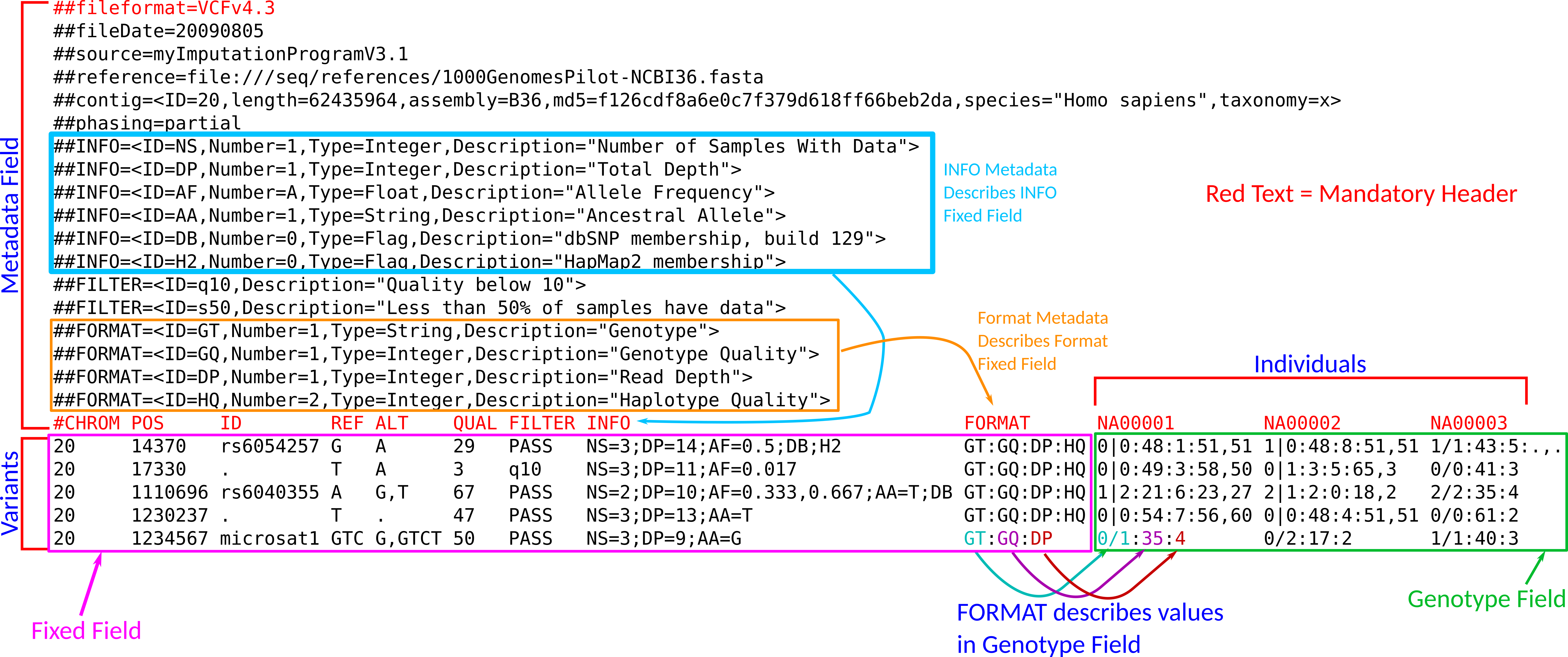
```
The VCF file is broken down as follows:
- A header with metadata (all lines beginning with ##). These describe properties of other parts of the file.
- Below the header, each row corresponds to a different variant. The columns can be subdivided as follows:
- A fixed field (columns CHROM, POS, ID, REF, ALT, QUAL, and FILTER). These contain information that are variant specific (i.e. are the same for all individuals).
- An info field (column INFO) that contains additional variant specific information.
- A genotype field, where the column names are the names of the individuals. In the above example, NA00001, NA00002, and NA00003, but these names may vary. The genotype field contains information that is specific for that individual at that locus.
The above file has five variants (five rows):
1. A SNP with one reference allele “G” and one alternative allele “A,”
2. Another SNP that did not pass quality checks, and so was filtered out.
3. A SNP with one reference allele “A” and two alternative alleles “G” and “T.”
4. A locus that is not a variant, because all individuals have a “T” there (this is called a monomorphic location)
5. A more complicated variant (called a “microsattelite”) where the reference allele is “GTC” and the two alternative alleles are “G” and “GTCT.”
VCF files can get really complicated, since they have to be able to store complicated differences between genomes. Here, we will just talk about basic information, which is what most people use it for anyway.
See the spec for more information: http://samtools.github.io/hts-specs/VCFv4.3.pdf

Metadata

The Metadata field is at the top of the VCF file and begins with ##.
The first line should say the version of VCF file format used (this is version 4.3).
There are some structured lines that must follow a certain format.
##INFO lines describe properties of the SNPs. You tell the VCF file the format of the INFO field through the metadata.
```
##INFO=<ID=ID,Number=number,Type=type,Description="description",Source="source",Version="version">
```
- ID: Should be the name of the INFO field.
- Number: The number values for an INFO field.
- Type: The base type of the field.
- The other arguments (Description, Source, Version) are just strings that don’t matter, and are optional.

The possible values of Number

Value	Descriptions
An integer, like `1` or `2`	The exact number of values
`A`	One value per alternate allele
`R`	One value for each allele
`G`	One value per genotype
`.`	Any number of possible values

The possible values of Type: Integer, Float, Flag, Character, or String.
- Float means decimal (kind of like doubles in R)
- Flag No value. Either it shows up or doesn’t.
##FORMAT lines describe the genotype fields that are possible.
```
##FORMAT=<ID=ID,Number=number,Type=type,Description="description">
```
- Number and Type have the same possibilities as the ##INFO line.

Fixed Field

Under the metadata, you have the the “fixed” field, where each line is a specific property of the variant.
The header looks like this (with one #)
```
#CHROM POS ID REF ALT QUAL FILTER INFO
```
CHROM: An identifier from the reference genome used to build the VCF file.
POS: Reference position on the chromosome.
ID: Name of the variant.
REF: Reference allele.
ALT: Alternative allele.
QUAL: Quality of the SNP. Officially, this is an estimate of $-10\log_{10}\text{Pr(call in ALT is wrong)}$. This is usually output by genotyping software.
FILTER: PASS if the variant passed filters placed on it by the genotyping software. Otherwise a code for why it failed to the filter.

INFO field

The INFO field is also a part of the fixed data, where each line is information on an entire variant. But it can contain a lot of different information, so I’ll treat it as an additional field.
INFO: Semicolon separated additional information.
The different keys in the INFO column are described by the ##INFO line in the metadata.

Table of common INFO keys (from VCF spec).

Key	Number	Type	Description
AA	1	String	Ancestral allele
AC	A	Integer	Allele count in genotypes, for each ALT allele, in the same order as listed
AD	R	Integer	Total read depth for each allele
ADF	R	Integer	Read depth for each allele on the forward strand
ADR	R	Integer	Read depth for each allele on the reverse strand
AF	A	Float	Allele frequency for each ALT allele in the same order as listed (estimated from primary data, not called genotypes)
AN	1	Integer	Total number of alleles in called genotypes
BQ	1	Float	RMS base quality
CIGAR	A	String	Cigar string describing how to align an alternate allele to the reference allele
DB	0	Flag	dbSNP membership
DP	1	Integer	Combined depth across samples
END	1	Integer	End position on CHROM (used with symbolic alleles; see below)
H2	0	Flag	HapMap2 membership
H3	0	Flag	HapMap3 membership
MQ	1	Float	RMS mapping quality
MQ0	1	Integer	Number of MAPQ == 0 reads
NS	1	Integer	Number of samples with data
SB	4	Integer	Strand bias
SOMATIC	0	Flag	Somatic mutation (for cancer genomics)
VALIDATED	0	Flag	Validated by follow-up experiment
1000G	0	Flag	1000 Genomes membership

Genotype Fields

Genotype information according to a VCF file is a property of an individual at a locus.
This is different from the Fixed field. The Fixed field has information on variants (same across individuals). The Genotype field has information that differs based on both variants and individuals.
The genotype field for each sample is colon separated.
The FORMAT column provides the order of the genotypes.
The ##FORMAT line in the metadata provides information on what the genotypes are.

Common genotype keys (from VCF spec), with bold for the ones I see most often:

Field	Number	Type	Description
AA	A	Integer	Read depth for alternative allele
AD	R	Integer	Read depth for each allele
ADF	R	Integer	Read depth for each allele on the forward strand
ADR	R	Integer	Read depth for each allele on the reverse strand
DP	1	Integer	Read depth
DS	1	Float	Posterior mean genotype
EC	A	Integer	Expected alternate allele counts
FT	1	String	Filter indicating if this genotype was “called”
GL	G	Float Genotype likelihoods
GP	G	Float Genotype posterior probabilities
GQ	1	Integer	Conditional genotype quality
GT	1	String	Genotype, with”`/`” meaning unphased and “`\|`” meaning phased
HQ	2	Integer	Haplotype quality
MQ	1	Integer	RMS mapping quality
PL	G	Integer	Phred-scaled genotype likelihoods rounded to the closest integer
PP	G	Integer	Phred-scaled genotype posterior probabilities rounded to the closest integer
PQ	1	Integer	Phasing quality
PS	1	Integer	Phase set
RA	1	Integer	Read depth for reference allele

VCF File Exercises

The following is a small part of a VCF file from Euclide et al. (2020), downloaded from <doi:10.5061/dryad.3mq4631>.

##fileformat=VCFv4.2
##fileDate=20180809
##source="Stacks v1.46"
##INFO=<ID=NS,Number=1,Type=Integer,Description="Number of Samples With Data">
##INFO=<ID=AF,Number=.,Type=Float,Description="Allele Frequency">
##FORMAT=<ID=GT,Number=1,Type=String,Description="Genotype">
##FORMAT=<ID=DP,Number=1,Type=Integer,Description="Read Depth">
##FORMAT=<ID=AD,Number=R,Type=Integer,Description="Allele Depth">
##INFO=<ID=locori,Number=1,Type=Character,Description="Orientation the corresponding Stacks locus aligns in">
#CHROM  POS   ID     REF  ALT  QUAL  FILTER  INFO                      FORMAT    LakeW_17-03702.1  Medici_17-13201.1  Medici_17-13202.1  Medici_17-13203.1  Medici_17-13204.1  
un      1358  10_96  A    G    .     PASS    NS=148;AF=0.057;locori=p  GT:DP:AD  0/0:12:12,0       0/0:30:30,0        0/0:17:17,0        0/0:16:16,0        0/0:20:20,0
un      2167  16_65  G    A    .     PASS    NS=122;AF=0.307;locori=p  GT:DP:AD  0/0:7:7,0         0/1:22:11,11       0/1:11:4,7         0/0:15:15,0        1/1:15:0,15 
un      2837  21_35  T    C    .     PASS    NS=132;AF=0.273;locori=p  GT:DP:AD  0/0:5:5,0         0/1:22:12,10       0/0:10:10,0        1/1:12:0,12        0/1:17:8,9

What are the reference alleles for the three loci?
What are the alternative alleles for the three loci?
What are the estimated genotypes at the three loci for Medici_17-13204.1?
What fraction of Medici_17-13202.1’s reads were “A” at locus 16_65?
What is the estimated allele frequency at locus 16_65?
When were these data created?

VariantAnnotation

The {VariantAnnotation} package provides an S4 object that has a slot for each field from a VCF file.`

Let’s load in an example VCF file that comes with the package (using readVcf().

fl <- system.file("extdata", "chr22.vcf.gz", package="VariantAnnotation")
vcf <- readVcf(fl, "hg19")
vcf

## class: CollapsedVCF 
## dim: 10376 5 
## rowRanges(vcf):
##   GRanges with 5 metadata columns: paramRangeID, REF, ALT, QUAL, FILTER
## info(vcf):
##   DataFrame with 22 columns: LDAF, AVGPOST, RSQ, ERATE, THETA, CIEND, CIPOS,...
## info(header(vcf)):
##              Number Type    Description                                        
##    LDAF      1      Float   MLE Allele Frequency Accounting for LD             
##    AVGPOST   1      Float   Average posterior probability from MaCH/Thunder    
##    RSQ       1      Float   Genotype imputation quality from MaCH/Thunder      
##    ERATE     1      Float   Per-marker Mutation rate from MaCH/Thunder         
##    THETA     1      Float   Per-marker Transition rate from MaCH/Thunder       
##    CIEND     2      Integer Confidence interval around END for imprecise var...
##    CIPOS     2      Integer Confidence interval around POS for imprecise var...
##    END       1      Integer End position of the variant described in this re...
##    HOMLEN    .      Integer Length of base pair identical micro-homology at ...
##    HOMSEQ    .      String  Sequence of base pair identical micro-homology a...
##    SVLEN     1      Integer Difference in length between REF and ALT alleles   
##    SVTYPE    1      String  Type of structural variant                         
##    AC        .      Integer Alternate Allele Count                             
##    AN        1      Integer Total Allele Count                                 
##    AA        1      String  Ancestral Allele, ftp://ftp.1000genomes.ebi.ac.u...
##    AF        1      Float   Global Allele Frequency based on AC/AN             
##    AMR_AF    1      Float   Allele Frequency for samples from AMR based on A...
##    ASN_AF    1      Float   Allele Frequency for samples from ASN based on A...
##    AFR_AF    1      Float   Allele Frequency for samples from AFR based on A...
##    EUR_AF    1      Float   Allele Frequency for samples from EUR based on A...
##    VT        1      String  indicates what type of variant the line represents 
##    SNPSOURCE .      String  indicates if a snp was called when analysing the...
## geno(vcf):
##   List of length 3: GT, DS, GL
## geno(header(vcf)):
##       Number Type   Description                      
##    GT 1      String Genotype                         
##    DS 1      Float  Genotype dosage from MaCH/Thunder
##    GL G      Float  Genotype Likelihoods

A quick view of the different slots can be seen with header()

header(vcf)

## class: VCFHeader 
## samples(5): HG00096 HG00097 HG00099 HG00100 HG00101
## meta(1): fileformat
## fixed(2): FILTER ALT
## info(22): LDAF AVGPOST ... VT SNPSOURCE
## geno(3): GT DS GL

`metadata` slot

A list having header information. This is mostly arbitrary information.

metadata(vcf)

## $header
## class: VCFHeader 
## samples(5): HG00096 HG00097 HG00099 HG00100 HG00101
## meta(1): fileformat
## fixed(2): FILTER ALT
## info(22): LDAF AVGPOST ... VT SNPSOURCE
## geno(3): GT DS GL

This VCF only has a metadata list of length 1, where that element is the header.

header(vcf)

## class: VCFHeader 
## samples(5): HG00096 HG00097 HG00099 HG00100 HG00101
## meta(1): fileformat
## fixed(2): FILTER ALT
## info(22): LDAF AVGPOST ... VT SNPSOURCE
## geno(3): GT DS GL

`VCFHeader`

The header is actually a new S4 class called VCFHeader which contains all of the information from the metadata of the VCF file (everything that begins with ##).
The slots are
- @reference: Arbitrary character vector with names of reference sequences.
- @samples: A character vector with the sample names. This should be the same as the row.names from the @colData slot of the VCF object.
- @header: A DataFrameList with the following elements:
  - fileformat: A DataFrame that looks like this:
```
fileformat = DataFrame(
  Value = "VCFv4.3",
  row.names = "fileformat"
)
```
  - INFO: A DataFrame with three columns (Number, Type, and Description), and row.names corresponding to the available info fields. If there are no info fields, just put down
```
INFO = DataFrame(
  Number = character(),
  Type = character(),
  Description = character()
)
```
  - FORMAT: A DataFrame with three columns (Number, Type, and Description), and row.names corresponding to the available geno fields.
  - QUAL: An optional DataFrame with a single column called Description.
  - FILTER: An optional DataFrame with a single column called Description.
  - ALT: An optional DataFrame with a single column called Description.
  - REF: An optional DataFrame with a single column called Description.
The constructor is VCFHeader().

You can get and set these values with fixed(), info(), geno(), samples(), and reference().

samples(header(vcf))

## [1] "HG00096" "HG00097" "HG00099" "HG00100" "HG00101"

reference(header(vcf))

## character(0)

fixed(header(vcf))

## DataFrameList of length 2
## names(2): FILTER ALT

info(header(vcf))

## DataFrame with 22 rows and 3 columns
##                Number        Type            Description
##           <character> <character>            <character>
## LDAF                1       Float MLE Allele Frequency..
## AVGPOST             1       Float Average posterior pr..
## RSQ                 1       Float Genotype imputation ..
## ERATE               1       Float Per-marker Mutation ..
## THETA               1       Float Per-marker Transitio..
## ...               ...         ...                    ...
## ASN_AF              1       Float Allele Frequency for..
## AFR_AF              1       Float Allele Frequency for..
## EUR_AF              1       Float Allele Frequency for..
## VT                  1      String indicates what type ..
## SNPSOURCE           .      String indicates if a snp w..

geno(header(vcf))

## DataFrame with 3 rows and 3 columns
##         Number        Type            Description
##    <character> <character>            <character>
## GT           1      String               Genotype
## DS           1       Float Genotype dosage from..
## GL           G       Float   Genotype Likelihoods

NOTE: A DataFrameList is another S4 object from {IRanges} that acts as just a list of DataFrame objects. You can construct one with

DataFrameList(
  x = DataFrame(a = c(1,2,3)),
  y = DataFrame(b = c("A", "B"),
                d = 4:5)
  )

## DataFrameList of length 2
## names(2): x y

`fixed` slot:

This contains information from the REF, ALT, QUAL, and FILTER columns from the VCF file.

fixed(vcf)

## DataFrame with 10376 rows and 4 columns
##                  REF                ALT      QUAL      FILTER
##       <DNAStringSet> <DNAStringSetList> <numeric> <character>
## 1                  A                  G       100        PASS
## 2                  C                  T       100        PASS
## 3                  G                  A       100        PASS
## 4                  C                  T       100        PASS
## 5                  C                  T       100        PASS
## ...              ...                ...       ...         ...
## 10372              A                  G       100        PASS
## 10373              A                  G       100        PASS
## 10374              A                  G       100        PASS
## 10375              G                  A       100        PASS
## 10376              G                  C       100        PASS

REF: DNAStringSet object. This contains the reference alleles at each locus. You can access it with ref()

ref(vcf)

## DNAStringSet object of length 10376:
##         width seq
##     [1]     1 A
##     [2]     1 C
##     [3]     1 G
##     [4]     1 C
##     [5]     1 C
##     ...   ... ...
## [10372]     1 A
## [10373]     1 A
## [10374]     1 A
## [10375]     1 G
## [10376]     1 G

ALT: DNAStringSetList object. Each element is a DNAStringSet containing the alternative alleles at each locus. In this case, there is only one alternative allele at every locus, but multiple alternative alleles are possible. You can access it with alt()
```
alt(vcf)
```
```
## DNAStringSetList of length 10376
## [[1]] G
## [[2]] T
## [[3]] A
## [[4]] T
## [[5]] T
## [[6]] A
## [[7]] C
## [[8]] A
## [[9]] A
## [[10]] C
## ...
## <10366 more elements>
```
```
all(lengths(alt(vcf)) == 1)
```
```
## [1] TRUE
```
QUAL: Numeric vector. Again, this is $-10\log_{10}\text{Pr(call in ALT is wrong)}$. You can access this with qual()
```
qual(vcf) |>
  head()
```
```
## [1] 100 100 100 100 100 100
```
FILTER: Character vector. Again, this is either "PASS" or a code for why it failed the filter.

`rowRanges` slot

A GRanges object, describing genomic locations of variant along with annotations.

rowRanges(vcf)

## GRanges object with 10376 ranges and 5 metadata columns:
##               seqnames    ranges strand | paramRangeID            REF
##                  <Rle> <IRanges>  <Rle> |     <factor> <DNAStringSet>
##     rs7410291       22  50300078      * |           NA              A
##   rs147922003       22  50300086      * |           NA              C
##   rs114143073       22  50300101      * |           NA              G
##   rs141778433       22  50300113      * |           NA              C
##   rs182170314       22  50300166      * |           NA              C
##           ...      ...       ...    ... .          ...            ...
##   rs187302552       22  50999536      * |           NA              A
##     rs9628178       22  50999538      * |           NA              A
##     rs5770892       22  50999681      * |           NA              A
##   rs144055359       22  50999830      * |           NA              G
##   rs114526001       22  50999964      * |           NA              G
##                              ALT      QUAL      FILTER
##               <DNAStringSetList> <numeric> <character>
##     rs7410291                  G       100        PASS
##   rs147922003                  T       100        PASS
##   rs114143073                  A       100        PASS
##   rs141778433                  T       100        PASS
##   rs182170314                  T       100        PASS
##           ...                ...       ...         ...
##   rs187302552                  G       100        PASS
##     rs9628178                  G       100        PASS
##     rs5770892                  G       100        PASS
##   rs144055359                  A       100        PASS
##   rs114526001                  C       100        PASS
##   -------
##   seqinfo: 1 sequence from hg19 genome; no seqlengths

You can access the IRanges object with genomic locations by the ranges() method.

ranges(vcf)

## IRanges object with 10376 ranges and 0 metadata columns:
##                   start       end     width
##               <integer> <integer> <integer>
##     rs7410291  50300078  50300078         1
##   rs147922003  50300086  50300086         1
##   rs114143073  50300101  50300101         1
##   rs141778433  50300113  50300113         1
##   rs182170314  50300166  50300166         1
##           ...       ...       ...       ...
##   rs187302552  50999536  50999536         1
##     rs9628178  50999538  50999538         1
##     rs5770892  50999681  50999681         1
##   rs144055359  50999830  50999830         1
##   rs114526001  50999964  50999964         1

Because these are all SNPs, all of the ranges are length 1.
This information comes from the POS column of the VCF and the sequence of REF.

`info` slot

DataFrame object with information on each variant.
```
info(vcf)
```
Each of those columns are a different INFO field described above.

You can get a description of the info fields by

info(header(vcf))

## DataFrame with 22 rows and 3 columns
##                Number        Type            Description
##           <character> <character>            <character>
## LDAF                1       Float MLE Allele Frequency..
## AVGPOST             1       Float Average posterior pr..
## RSQ                 1       Float Genotype imputation ..
## ERATE               1       Float Per-marker Mutation ..
## THETA               1       Float Per-marker Transitio..
## ...               ...         ...                    ...
## ASN_AF              1       Float Allele Frequency for..
## AFR_AF              1       Float Allele Frequency for..
## EUR_AF              1       Float Allele Frequency for..
## VT                  1      String indicates what type ..
## SNPSOURCE           .      String indicates if a snp w..

`colData` slot

A DataFrame object describing sample information.

colData(vcf)

## DataFrame with 5 rows and 1 column
##           Samples
##         <integer>
## HG00096         1
## HG00097         2
## HG00099         3
## HG00100         4
## HG00101         5

Right now, this just has the sample number.
The row.names should be the names of the samples. These should be the same as the sample names from the VCFHeader.

`geno` slot

A SimpleList of matrix or array objects, containing the genotype data
```
geno(vcf)
```
```
## List of length 3
## names(3): GT DS GL
```
The different genotype data possible are described above.
In this example, we have fields GT (the genotype), DS (genotype dosage, aka posterior mean genotype), and GL (genotype likelihoods).

You can always get a description of the genotype fields with:

geno(header(vcf))

## DataFrame with 3 rows and 3 columns
##         Number        Type            Description
##    <character> <character>            <character>
## GT           1      String               Genotype
## DS           1       Float Genotype dosage from..
## GL           G       Float   Genotype Likelihoods

You can access these different genotype fields by
```
geno(vcf)$GL
```

Filtering

There are many operations available to filer loci using the VCF class.
Get first twenty rows:
```
dim(vcf)
vcf[1:20, ]
```

Saving

Use writeVcf() to save a VCF file.

`{VariantAnnotation}` Exercises

The data in the VCF file https://dcgerard.github.io/advancedr/data/wal_CF.vcf contain a very small subset of the data from Euclide et al. (2020), downloaded from <doi:10.5061/dryad.3mq4631>. Let’s use the {VariantAnnotation} package to play around with it.

Read these data into R.
Are all loci biallelic?
It is common to filter out loci that have too low or too high an allele frequency. What proportion of loci have allele frequencies between 0.05 and 0.95.
Filter the loci so that you only have loci with allele frequencies between 0.05 and 0.95.
Recall that AD is a matrix list, where each element is a numeric vector containing the read depth for each allele for that individual at that locus. Create an integer matrix called AA that contains the read depth for just the alternative allele. Make sure column and row names match those of the other geno elements.
If your VCF object is called vcf_obj, modify geno(header(vcf_obj)) so that your genotype field now contains an AA element.
Write your VCF object to a file called “vcf_new.vcf.”

References

Euclide, Peter T., Garrett J. McKinney, Matthew Bootsma, Charlene Tarsa, Mariah H. Meek, and Wesley A. Larson. 2020. “Attack of the PCR Clones: Rates of Clonality Have Little Effect on RAD-Seq Genotype Calls.” Molecular Ecology Resources 20 (1): 66–78. https://doi.org/10.1111/1755-0998.13087.

This work is licensed under a Creative Commons Attribution-NonCommercial 4.0 International License.

S4 and Bioconductor

David Gerard

2022-02-07

Learning Objectives

Motivation

Bioconductor Setup

Basic Objects

`SimpleList`

`DataFrame`

`CharacterList`, `NumericList`, `IntegerList`, `LogicalList`

`Rle`

`IRanges`

`GRanges`

`DNAString`

`DNAStringSet`

`DNAStringSetList`

Basic Data Exercises

VCF Files

VCF Diagram

Metadata

Fixed Field

INFO field

Genotype Fields

VCF File Exercises

VariantAnnotation

`metadata` slot

`VCFHeader`

`fixed` slot:

`rowRanges` slot

`info` slot

`colData` slot

`geno` slot

Filtering

Saving

`{VariantAnnotation}` Exercises

References

S4 and Bioconductor

David Gerard

2022-02-07

Learning Objectives

Motivation

Bioconductor Setup

Basic Objects

SimpleList

DataFrame

CharacterList, NumericList, IntegerList, LogicalList

Rle

IRanges

GRanges

DNAString

DNAStringSet

DNAStringSetList

Basic Data Exercises

VCF Files

VCF Diagram

Metadata

Fixed Field

INFO field

Genotype Fields

VCF File Exercises

VariantAnnotation

metadata slot

VCFHeader

fixed slot:

rowRanges slot

info slot

colData slot

geno slot

Filtering

Saving

{VariantAnnotation} Exercises

References

`SimpleList`

`DataFrame`

`CharacterList`, `NumericList`, `IntegerList`, `LogicalList`

`Rle`

`IRanges`

`GRanges`

`DNAString`

`DNAStringSet`

`DNAStringSetList`

`metadata` slot

`VCFHeader`

`fixed` slot:

`rowRanges` slot

`info` slot

`colData` slot

`geno` slot

`{VariantAnnotation}` Exercises