Formulas

Learning Objectives

• Overview of Formulas
• {lme4} Vignette

Motivation

• A formula is a basic data structure in R.

• Whenever you have used a tilde (~), you have used a formula.

• formulas are used in t.test(), lm(), glm(), lme4::lmer(), lme4::nlmer(), facet_grid(), facet_wrap(), purrr::map() and relatives, reshape2::acast(), aggregate(), etc…

• We will learn about

  1. The structure of a formula
  2. The syntax for formulas.
  3. Functions to work with formulas

Formula Creation

• Formulas are data structures that consist of

  1. A left-hand side (LHS) call
  2. A right-hand side (RHS) call
  3. An environment.

• So they are two calls with an environment attached (like a quosure).

  • Formally, they are expressions of length 3, where the first element is the function call ~, the second element is the LHS, and the third element is the RHS. They have a .Environment attribute.

• You commonly create a formula with a tilde ~.

  f1 <- y ~ x + z
  class(f1)

  ## [1] "formula"

  typeof(f1) ## built on calls

  ## [1] "language"

  attributes(f1)

  ## $class
  ## [1] "formula"
  ## 
  ## $.Environment
  ## <environment: R_GlobalEnv>

  length(f1)

  ## [1] 3

  f1[[1]]

  ## `~`

  f1[[2]]

  ## y

  f1[[3]]

  ## x + z

• Test if an object is a formula with rlang::is_formula().

  rlang::is_formula(f1)

  ## [1] TRUE

• The ~ uses the call environment as the formula environment. You can specify other environments using rlang::new_formula().

  e <- rlang::env()
  rlang::new_formula(lhs = rlang::expr(y), rhs = rlang::expr(x), env = e)

  ## y ~ x
  ## <environment: 0x55eff68468e0>

• You can have one-sided formulas with only a RHS, in which case they have length 2.

  f2 <- ~ x + y
  f2

  ## ~x + y

  length(f2)

  ## [1] 2

Formula Syntax

• In modeling contexts, the LHS contains the name of the response variable.

• The RHS contains the predictor variables that are linearly related to the response (up to some link function).

• Terms separated by a + indicate main effects.

  mpg ~ wt + drat + hp

  ## mpg ~ wt + drat + hp

  \[ \text{mpg} = \beta_0 + \beta_1\text{wt} + \beta_2\text{drat} + \beta_3 \text{hp} \]

• Terms separated by a : indicate interaction effects.

  mpg ~ wt:drat + hp

  ## mpg ~ wt:drat + hp

  \[ \text{mpg} = \beta_0 + \beta_{12}\text{wt}\times\text{drat} + \beta_3 \text{hp} \]

• Terms separated by a * indicate interaction and main effects.

  mpg ~ wt * drat + hp

  ## mpg ~ wt * drat + hp

  \[ \text{mpg} = \beta_0 + \beta_1\text{wt} + \beta_2\text{drat} + \beta_{12}\text{wt}\times\text{drat} + \beta_3 \text{hp} \]

• Note that a*a does not give you a quadratic term in a.

  lm(mpg ~ wt * wt, data = mtcars)

  ## 
  ## Call:
  ## lm(formula = mpg ~ wt * wt, data = mtcars)
  ## 
  ## Coefficients:
  ## (Intercept)           wt  
  ##       37.29        -5.34

• The ^ indicates crossing to a provided degree.

  mpg ~ (wt + drat + hp)^2

  ## mpg ~ (wt + drat + hp)^2

  is the same as

  mpg ~ (wt + drat + hp) * (wt + drat + hp)

  ## mpg ~ (wt + drat + hp) * (wt + drat + hp)

  which is the same as

  mpg ~ wt + drat + hp + wt:drat + wt:hp + drat:hp

  ## mpg ~ wt + drat + hp + wt:drat + wt:hp + drat:hp

• The - operator removes terms.

  mpg ~ wt*drat + hp - wt

  ## mpg ~ wt * drat + hp - wt

  is the same as

  mpg ~ drat + wt:drat + hp

  ## mpg ~ drat + wt:drat + hp

• The 1 is an implicit variable for the \(y\)-intercept. You can remove it via subtraction

  mpg ~ mpg + drat + hp - 1

  ## mpg ~ mpg + drat + hp - 1

  \[ \text{mpg} = \beta_1\text{wt} + \beta_2\text{drat} + \beta_3 \text{hp} \]

{lme4}

• Mixed models allow for model parameters to be treated as random variables (e.g. random slopes or intercepts).

• You do this to control for correlation between samples. E.g.

  • Many observations collected on the same individuals.
  • Observations are a part of a hierarchy. E.g. data collected on students who belong to schools who belong to districts.

• Lots of folks prefer treating effects as random (as opposed to fixed) when they are interested as the population as a whole more than specific values of a covariate.

• E.g. in a study on sleep deprivation, Researchers measured reaction times for individuals after so many days of sleep deprivation.

  library(ggplot2)
  data("sleepstudy", package = "lme4")
  ggplot(sleepstudy, aes(x = Days, y = Reaction)) +
    facet_wrap(. ~ Subject) +
    geom_point() +
    geom_smooth(method = "lm", se = FALSE)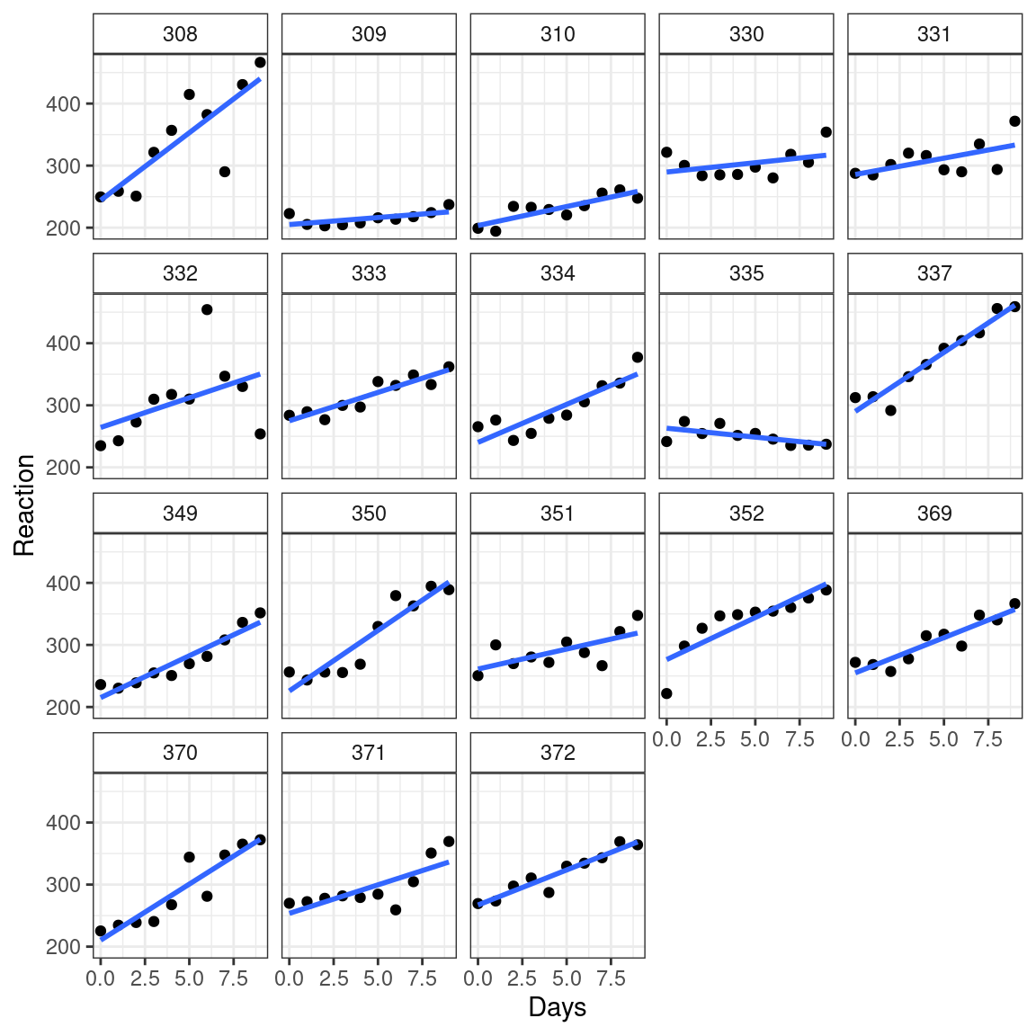

  

• Each subject has different slopes and intercepts.

• We don’t care about the slopes and intercepts for each subject, but we want to account for correlation within subjects.

• So we might consider the slope and intercept of each subject to be random.

• Folks don’t just include fixed effects for subject because it would use a lot more degrees of freedom (this is a cynical view).

• To specify just random intercepts (different for each subject), do

  lm1 <- lme4::lmer(Reaction ~ Days + (1 | Subject), data = sleepstudy)

• To specify random slopes (different slope on Day for each subject), do

  lm2 <- lme4::lmer(Reaction ~ Days + (Days | Subject), data = sleepstudy)

• Let

  • \(y_i\) be the reaction time for observation \(i\).
  • \(x_i\) be the day for observation \(i\).
  • \(z_{ij}\) be an indicator for subject \(j\).

• Then lm1 fit the model \[ y_i = \beta_0 + \beta_1x_i + \sum_{j=1}^{18}\alpha_{0j}z_{ij} + \epsilon_i\\ \alpha_{0j} \overset{iid}{\sim} N(0, \sigma^2)\\ \epsilon_i \overset{iid}{\sim} N(0, \tau^2) \]

• lm2 fit the model \[ y_i = \beta_0 + \beta_1x_i + \sum_{j=1}^{18}\alpha_{0j}z_{ij} + \sum_{j=1}^{18}\alpha_{1j}x_iz_{ij} + \epsilon_i\\ (\alpha_{0j},\alpha_{1j}) \overset{iid}{\sim} N_{2}(0, \Sigma)\\ \epsilon_i \overset{iid}{\sim} N(0, \tau^2) \]

• The idea is that we specify the random effects with the parentheses. The left of the | is the explanatory variable to model a relationship with the response, to the right of the pipe is the grouping factor that is assumed to be random.

• E.g., in lm1 the the \(y\)-intercept was different for each subject.

• E.g., in lm2 the the slope of Day and \(y\)-intercept was different for each subject.

• Here are the common formulations (Table 2 from {lme4} vignette):

  Formula	Meaning
  y ~ (1 | g)	Random intercept with fixed mean.
  y ~ (1 | g1/g2) or y ~ (1 | g1) + (1 | g1:g2)	Intercept varying among g1 and g2 within g1.
  y ~ (1 | g1) + (1 | g2)	Intercept varying among g1 and g2.
  y ~ x + (x | g)	Correlated random intercept and slope

  • y is the response, x is the explanatory, and g g1 g1 are grouping variables.

Working with Formulas

• all.vars() will return a character vector of variable names used in the formula

  f <- mpg ~ wt:drat + hp
  all.vars(f)

  ## [1] "mpg"  "wt"   "drat" "hp"

• Add variables to a formula with update.formula(). You use a . to represent everything on LHS or RHS.

  f <- y ~ x
  f <- update.formula(old = f, new = ~ . + z)
  f

  ## y ~ x + z

• model.frame() will take as input a formula and a data frame and will create a new data frame containing all of the variables involved in the formula. If the variables are not in the data frame, R will look for them in the formula environment.

  f <- mpg ~ wt:drat + hp
  mfout <- model.frame(formula = f, data = mtcars)
  head(mfout)

  ##                    mpg    wt drat  hp
  ## Mazda RX4         21.0 2.620 3.90 110
  ## Mazda RX4 Wag     21.0 2.875 3.90 110
  ## Datsun 710        22.8 2.320 3.85  93
  ## Hornet 4 Drive    21.4 3.215 3.08 110
  ## Hornet Sportabout 18.7 3.440 3.15 175
  ## Valiant           18.1 3.460 2.76 105

  attributes(mfout)

  ## $names
  ## [1] "mpg"  "wt"   "drat" "hp"  
  ## 
  ## $terms
  ## mpg ~ wt:drat + hp
  ## attr(,"variables")
  ## list(mpg, wt, drat, hp)
  ## attr(,"factors")
  ##      hp wt:drat
  ## mpg   0       0
  ## wt    0       2
  ## drat  0       2
  ## hp    1       0
  ## attr(,"term.labels")
  ## [1] "hp"      "wt:drat"
  ## attr(,"order")
  ## [1] 1 2
  ## attr(,"intercept")
  ## [1] 1
  ## attr(,"response")
  ## [1] 1
  ## attr(,".Environment")
  ## <environment: R_GlobalEnv>
  ## attr(,"predvars")
  ## list(mpg, wt, drat, hp)
  ## attr(,"dataClasses")
  ##       mpg        wt      drat        hp 
  ## "numeric" "numeric" "numeric" "numeric" 
  ## 
  ## $row.names
  ##  [1] "Mazda RX4"           "Mazda RX4 Wag"       "Datsun 710"         
  ##  [4] "Hornet 4 Drive"      "Hornet Sportabout"   "Valiant"            
  ##  [7] "Duster 360"          "Merc 240D"           "Merc 230"           
  ## [10] "Merc 280"            "Merc 280C"           "Merc 450SE"         
  ## [13] "Merc 450SL"          "Merc 450SLC"         "Cadillac Fleetwood" 
  ## [16] "Lincoln Continental" "Chrysler Imperial"   "Fiat 128"           
  ## [19] "Honda Civic"         "Toyota Corolla"      "Toyota Corona"      
  ## [22] "Dodge Challenger"    "AMC Javelin"         "Camaro Z28"         
  ## [25] "Pontiac Firebird"    "Fiat X1-9"           "Porsche 914-2"      
  ## [28] "Lotus Europa"        "Ford Pantera L"      "Ferrari Dino"       
  ## [31] "Maserati Bora"       "Volvo 142E"         
  ## 
  ## $class
  ## [1] "data.frame"

• The order of the variables are:

  1. The response variable is the first column
  2. All of the predictor variables are in subsequent columns.

• The resulting data frame has a terms attribute, which you can extract via terms().

  terms(mfout)

  ## mpg ~ wt:drat + hp
  ## attr(,"variables")
  ## list(mpg, wt, drat, hp)
  ## attr(,"factors")
  ##      hp wt:drat
  ## mpg   0       0
  ## wt    0       2
  ## drat  0       2
  ## hp    1       0
  ## attr(,"term.labels")
  ## [1] "hp"      "wt:drat"
  ## attr(,"order")
  ## [1] 1 2
  ## attr(,"intercept")
  ## [1] 1
  ## attr(,"response")
  ## [1] 1
  ## attr(,".Environment")
  ## <environment: R_GlobalEnv>
  ## attr(,"predvars")
  ## list(mpg, wt, drat, hp)
  ## attr(,"dataClasses")
  ##       mpg        wt      drat        hp 
  ## "numeric" "numeric" "numeric" "numeric"

• The terms object is the supplied formula with attributes that can be used to make the model matrix.

• The terms object can be read about via

  ?terms.object

• You can do manipulations on terms objects with delete.response(), drop.terms(), and reformulate().

• model.matrix() can be used to create the design matrix (the \(X\) matrix from regression).

  X <- model.matrix(object = f, data = mtcars)
  head(X)

  ##                   (Intercept)  hp wt:drat
  ## Mazda RX4                   1 110  10.218
  ## Mazda RX4 Wag               1 110  11.213
  ## Datsun 710                  1  93   8.932
  ## Hornet 4 Drive              1 110   9.902
  ## Hornet Sportabout           1 175  10.836
  ## Valiant                     1 105   9.550

• You either provide it a data frame to look for variables, or it looks for variables in the formula environment.

• model.matrix() basically evaluates interactions, and includes the intercept.

• model.matrix() can also be used on the output of model.frame(). Just make sure to include the data argument.

  X <- model.matrix(object = mfout, data = mtcars)
  head(X)

  ##                   (Intercept)  hp wt:drat
  ## Mazda RX4                   1 110  10.218
  ## Mazda RX4 Wag               1 110  11.213
  ## Datsun 710                  1  93   8.932
  ## Hornet 4 Drive              1 110   9.902
  ## Hornet Sportabout           1 175  10.836
  ## Valiant                     1 105   9.550

• Use model.response() on the output of model.frame() to get the response vector matrix.

  y <- model.response(mfout)
  head(y)

  ##         Mazda RX4     Mazda RX4 Wag        Datsun 710    Hornet 4 Drive 
  ##              21.0              21.0              22.8              21.4 
  ## Hornet Sportabout           Valiant 
  ##              18.7              18.1

Using formulas in a function

1. Include formula and data arguments.
2. Use model.frame()
3. Extract the response vector (model.response()) and design matrix (model.matrix()) from the model frame.
4. Do what you want with those entities.

• Example:

  f <- function(formula, data) {
    stopifnot(rlang::is_formula(formula))
    mf <- model.frame(formula = formula, data = data)
    y <- model.response(mf)
    X <- model.matrix(object = mf, data = data)
    ## Continue with your method ...
  }

• Sometimes you want to treat the different explanatory variables differently. One way would be to (i) separate them by the pipe |, (ii) convert to a string, (iii) do string manipulation, (iv) then use as.formula() to coerce back to a formula.

  f <- mpg ~ wt + drat | am + hp
  chvec <- as.character(f)
  xvec <- strsplit(chvec[[3]], "\\|")[[1]]
  f1 <- as.formula(paste0(chvec[[2]], "~", xvec[[1]], "-1"))
  f2 <- as.formula(paste0(chvec[[2]], "~", xvec[[2]], "-1"))
  X1 <- model.matrix(object = f1, data = mtcars, intercept = FALSE)
  X2 <- model.matrix(object = f2, data = mtcars)
  f1

  ## mpg ~ wt + drat - 1

  f2

  ## mpg ~ am + hp - 1

  head(X1)

  ##                      wt drat
  ## Mazda RX4         2.620 3.90
  ## Mazda RX4 Wag     2.875 3.90
  ## Datsun 710        2.320 3.85
  ## Hornet 4 Drive    3.215 3.08
  ## Hornet Sportabout 3.440 3.15
  ## Valiant           3.460 2.76

  head(X2)

  ##                   am  hp
  ## Mazda RX4          1 110
  ## Mazda RX4 Wag      1 110
  ## Datsun 710         1  93
  ## Hornet 4 Drive     0 110
  ## Hornet Sportabout  0 175
  ## Valiant            0 105

{rlang} Formula Manipulation

• {rlang} has a lot of formula manipulation tools that aren’t useful for working with datasets, but are useful if you want to use formula’s as data structures in their own right.

• Create a new formula with rlang::new_formula().

  fnew <- rlang::new_formula(lhs = rlang::expr(y + w), rhs = rlang::expr(x + z))

• Test for formula with rlang::is_formula().

  rlang::is_formula(fnew)

  ## [1] TRUE

• Get or set the formula environment with rlang::f_env()

  rlang::f_env(fnew)

  ## <environment: R_GlobalEnv>

• Get or set the LHS with rlang::f_lhs()

  rlang::f_lhs(fnew)

  ## y + w

• Get or set the RHS with rlang::f_rhs()

  rlang::f_rhs(fnew)

  ## x + z

• Convert RHS to text with rlang::f_text()

  rlang::f_text(fnew)

  ## [1] "x + z"

New Functions

• ~ Create a formula using call environment.
• rlang::new_formula(): Create a formula using any other environment.
• rlang::is_formula(): Predicate for formula.
• terms.formula(): Extract terms from a formula.
• update.formula(): Add variables to a formula.
• all.vars(): Get variable names used in a formula.
• model.matrix(): Get design matrix.
• model.frame(): Get matrix of variables used in model.
• model.response(): Get the response matrix from the output of model.frame().
• as.formula(): Coerce to a formula.

---

This work is licensed under a Creative Commons Attribution-NonCommercial 4.0 International License.