A Brief Overview of Metaprogramming

Learning Objectives

• Overview of Metaprogramming.
• Learn a couple tricks.
• Required: Chapter 17 of Advanced R
• Optional: Hadley goes into a lot of depth in Chapters 18–21 of Advanced R. But we’ll just learn some common and simple use-cases.
  • Those chapters only need to be understood in great depth if you actually want to help contribute to the tidyverse.

Overview

• Metaprogramming refers to treating code as data. You can save code as a variable, modify the code with other code, then evaluate the code.

• In R, we call saved code expressions.

• You can use rlang::expr() to create an expression.

  my_exp <- rlang::expr(x + y)

• The result is an expression of type language

  typeof(my_exp)

  ## [1] "language"

• If we print out my_exp, we just see our code

  my_exp

  ## x + y

• We can evaluate it (make the code run and provide a result) with base::eval()

  x <- 10
  y <- 11
  base::eval(my_exp)

  ## [1] 21

• The main ideas of metaprogramming:

  1. Treat source code as data
  2. Possibly modify source code programattically,
  3. Evaluate source code in a given environment.

• R is one of the few popular languages that provides extensive support for metaprogramming, another one being Lisp (and its children).

• We will use {rlang} for manipulating expressions.

  library(rlang)

Types of Expressions

• When constants are captured, they are just returned as the constant that they are.

  x <- rlang::expr(2)
  typeof(x)

  ## [1] "double"

  y <- rlang::expr("two")
  typeof(y)

  ## [1] "character"

• Symbols are names of objects.

  y <- rlang::expr(x)
  x <- c(22, 11, 13)
  eval(y)

  ## [1] 22 11 13

  typeof(y)

  ## [1] "symbol"

• Calls are function calls. Base R calls these languages.

  y <- rlang::expr(sum(x))
  x <- c(22, 11, 13)
  eval(y)

  ## [1] 46

  typeof(y)

  ## [1] "language"

• Calls act a lot like lists, where you can access arguments with list-like operators.

  fun <- rlang::expr(f(x, y))
  fun

  ## f(x, y)

• The first element of a call is the function argument.

  fun[[1]]

  ## f

• Each additional element of a call is an argument.

  fun[[2]]

  ## x

  fun[[3]]

  ## y

• You can add new arguments by inserting symbols.

  fun[[4]] <- rlang::expr(z)
  fun

  ## f(x, y, z)

• You can make arguments have default values.

  fun$w <- 1
  fun

  ## f(x, y, z, w = 1)

• To create a call from expressions, use rlang::call2(). The first argument is the function name (in quotes, or as an expression), and subsequent arguments are expressions of arguments.

  x <- c(1, 2, 3)
  y <- rlang::expr(x)
  z <- rlang::call2("sum", y)
  z

  ## sum(x)

  eval(z)

  ## [1] 6

Capturing Code

• As we’ve seen, to capture code, use rlang::expr().

  x <- 10
  y <- 11
  myexp <- rlang::expr(x + y)
  myexp

  ## x + y

  eval(expr = myexp)

  ## [1] 21

• Capturing an expression directly from code is called quoting (e.g. from rlang::expr()).

• Converting a string to an expression is called parsing and can be done with rlang::parse_expr().

  my_exp2 <- rlang::parse_expr("x + y")
  eval(my_exp2)

  ## [1] 21

• Converting code to a string is called deparsing. You do this with rlang::expr_text()

  rlang::expr_text(my_exp2)

  ## [1] "x + y"

• There is unquoting, where you selectively evaluate part of the expression. You use !! (pronounced “bang-bang”) to unquote. So below, x is unquoted.

  x <- 10
  y <- 11
  rlang::expr(y + !!x)

  ## y + 10

  • Though, !! is an invention of {rlang}, so if you use base R expression methods it won’t work.

• To capture function arguments as an expression, you have to use rlang::enexpr() (for “enrich expr()”).

  capture_exp <- function(x) {
    newexp <- rlang::enexpr(arg = x)
    return(newexp)
  }
  abc <- capture_exp(a + b + c)
  abc

  ## a + b + c

  a <- 1
  b <- 2
  c <- 3
  eval(abc)

  ## [1] 6

• The reason is that if you use rlang::expr(x) it will just return the expression with x, not with the values of the argument that you pass it.

  capture_bad <- function(x) {
    newexp <- rlang::expr(expr = x)
    return(newexp)
  }
  capture_bad(a + b + c)

  ## x

• Use rlang::enxprs() to capture a list of all arguments in ...

  capall <- function(...) {
    all_args <- rlang::enexprs(...)
    return(all_args)
  }
  capall(x + y, y * 2)

  ## [[1]]
  ## x + y
  ## 
  ## [[2]]
  ## y * 2

• Typically, when you use enexprs(), you get a list of expressions. You can then work with each individually through a for-loop. E.g.

  evalall <- function(...) {
    dots <- rlang::enexprs(...)
    lval <- list()
    for (i in seq_along(dots)) {
      lval[[i]] <- eval(dots[[i]])
    }
    return(lval)
  }
  a <- 3
  b <- 2
  evalall(a + b, b^2)

  ## [[1]]
  ## [1] 5
  ## 
  ## [[2]]
  ## [1] 4

Evaluated versus Quoted Arguments

• Evaluated arguments are those whose values are used. E.g. in sum(x), the x values are being used, but the variable name x is not.

• Quoted arguments are those where the code is used. E.g. in library(rlang) we use the code rlang and not the value that rlang binds to.

• Lots of dplyr functions use quoted arguments (where they use expressions in terms of variable names).

• Exercise: Which are evaluated arguments and which are quoted arguments in the below function calls

  dplyr::filter(mtcars, mpg > 20, wt > 3)
  
  ggplot(mtcars, aes(x = wt, y = mpg)) +
    geom_point(col = "red")
  
  mtcars$mpg
  
  mtcars[["mpg"]]

Quosures

• The {rlang} team made a new data object called a quosure (quoting closure) that bundles an expression with an environment. This makes it so that you do not have ambiguity when you evaluate an expression in a different environment where you have variable bindings.

• E.g. the following is presents an issue of the user wanting a to be 10 but we have a being 1000.

  fun <- function(x) {
    a <- 1000
    x <- rlang::enexpr(x)
    eval(x)
  }
  a <- 10
  fun(a + 1)

  ## [1] 1001

• Using rlang::enquo() will create a “quosure” which also includes the function environment. You cannot use base::eval() with a quosure, so {rlang} proves rlang::eval_tidy().

  fun <- function(x) {
    a <- 1000
    x <- rlang::enquo(x)
    rlang::eval_tidy(x)
  }
  a <- 10
  fun(a + 1)

  ## [1] 11

• Quosures are mostly used when you use dots ... in a function argument and want to use that in conjunction with data masking (where you use a data frame like an environment). This is what most {dplyr} functions do. E.g. dplyr::filer() uses data masking with the .data like an environment and different predicates as the expressions. See the following help file for more information

  ?`topic-quosure`

Application: Capturing Argument Names

• If we come up with a cool new plotting function, we might want to have the axis names match the variable names. But this does not occur with the naive approach.

  plot_red <- function(x, y) {
    oldpar <- par(mar = c(2.4, 2.8, 1, 0) + 0.5, mgp = c(1.8, 0.6, 0), las = 1)
    on.exit(par(oldpar), add = TRUE)
  
    plot(x, y, col = "red")
  }
  plot_red(x = mtcars$wt, y = mtcars$mpg)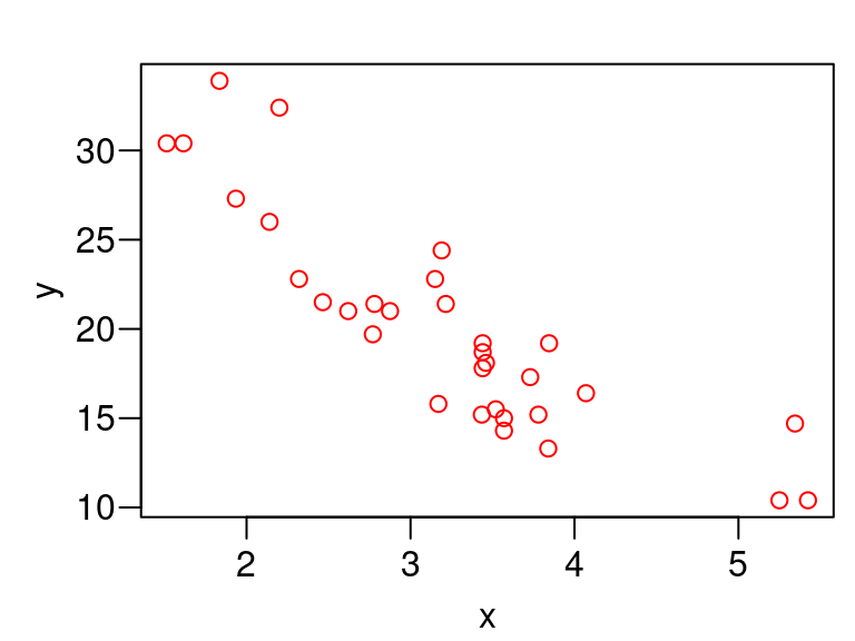

  

• We can do better by using quoted arguments, instead of evaluated arguments.

  plot_red <- function(x, y) {
    oldpar <- par(mar = c(2.4, 2.8, 1, 0) + 0.5, mgp = c(1.8, 0.6, 0), las = 1)
    on.exit(par(oldpar), add = TRUE)
  
    xexpr <- rlang::enexpr(x)
    yexpr <- rlang::enexpr(y)
    plot(x, y, col = "red", 
         xlab = rlang::expr_text(xexpr), 
         ylab = rlang::expr_text(yexpr))
  }
  plot_red(x = mtcars$wt, y = mtcars$mpg)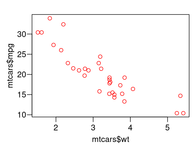

  

• But we can do even better than that by also having the user provide the data

  plot_red <- function(x, y, data) {
    oldpar <- par(mar = c(2.4, 2.8, 1, 0) + 0.5, mgp = c(1.8, 0.6, 0), las = 1)
    on.exit(par(oldpar), add = TRUE)
  
    xexpr <- rlang::enexpr(x)
    yexpr <- rlang::enexpr(y)
    plot(x = data[[xexpr]], 
         y = data[[yexpr]], 
         col = "red", 
         xlab = rlang::expr_text(xexpr), 
         ylab = rlang::expr_text(yexpr))
  }
  plot_red(x = wt, y = mpg, data = mtcars)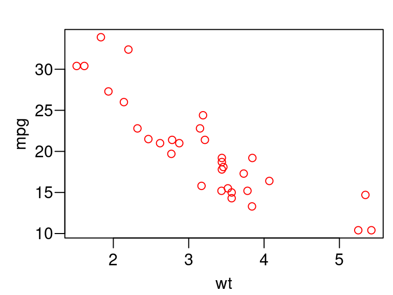

  

• This works because you can subset by an expression as well

  mtcars[[rlang::expr(mpg)]]

  ##  [1] 21.0 21.0 22.8 21.4 18.7 18.1 14.3 24.4 22.8 19.2 17.8 16.4 17.3 15.2 10.4
  ## [16] 10.4 14.7 32.4 30.4 33.9 21.5 15.5 15.2 13.3 19.2 27.3 26.0 30.4 15.8 19.7
  ## [31] 15.0 21.4

Application: Math Notation in Plots

• R has its own weird syntax for plotting mathematical equations.

• See the following help file for a full description:

  ?plotmath

• R uses expressions to implement mathematical notation in R.

• E.g. to write the following in R math

  \[ \sum_{i=1}^\infty x_i^2 + \beta_1 \]

  we would first create an expression using the R math notation:

  mathexp <- rlang::expr(sum(x[i]^2, i == 1, infinity) + beta[1])

• You can then use that expression in geom_text() or xlab() or whatever.

  plot.new()
  text(x = 0.5, y = 0.5, labels = mathexp, cex = 2)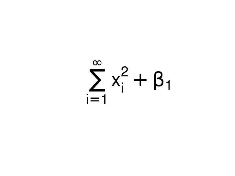

  

• What if you want to place the estimated slope of a regression on a graph?

  library(ggplot2)
  pl <- ggplot(mtcars, aes(x = wt, y = mpg)) +
    geom_point() +
    geom_smooth(method = "lm", se = FALSE)

• First, we calculate the OLS estimates:

  lmout <- lm(mpg ~ wt, data = mtcars)
  coefvec <- coef(lmout)
  coefvec

  ## (Intercept)          wt 
  ##      37.285      -5.344

• We could add the equation manually

  mathexp <- rlang::expr(hat(y)[i] == 37.2 - 5.3 * x[i])
  pl + annotate(geom = "text", x = 4.5, y = 30, label = mathexp)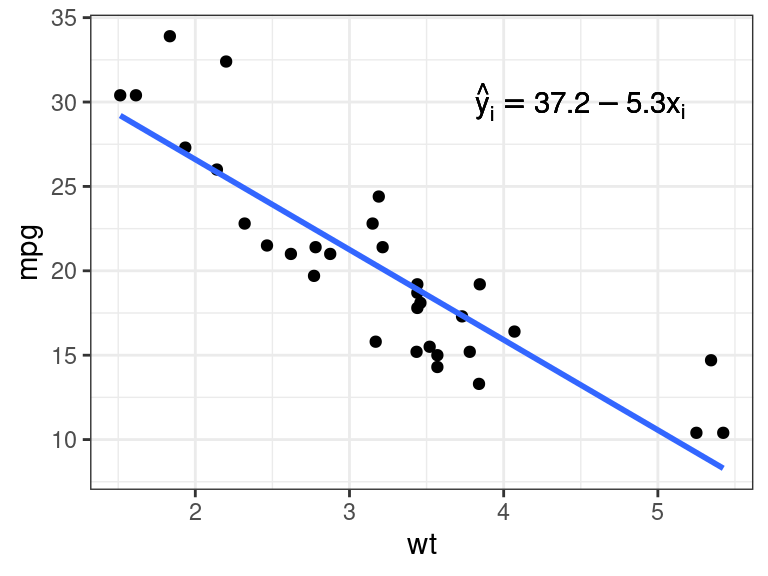

  

• However, this is prone to error (e.g., did you notice that I incorrectly rounded down to 37.2?)

• Just including the coefficient vectors won’t work.

  mathexp <- rlang::expr(hat(y)[i] == coefvec[[1]] - coefvec[[2]] * x[i])
  pl + annotate(geom = "text", x = 4.5, y = 30, label = mathexp)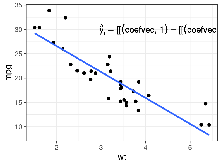

  

• Unquoting to the rescue! Just use !!.

  mathexp <- rlang::expr(hat(y)[i] == !!coefvec[[1]] - !!coefvec[[2]] * x[i])
  pl + annotate(geom = "text", x = 4.5, y = 30, label = mathexp)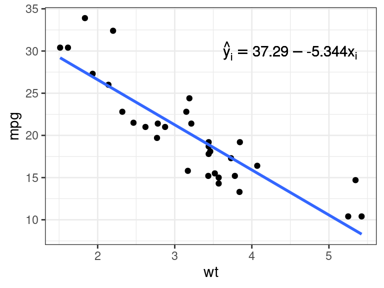

  

• If you want to plot more than one math equation, you need to use an expression vector, which is an object output by base::expression()

  evec <- expression(x^2, sqrt(y))
  plot(x = c(1, 2), y = c(1, 2), type = "n", xlim = c(0, 3), ylim = c(0, 3))
  text(x = c(1, 2), y = c(1, 2), labels = evec)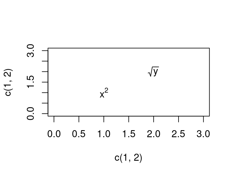

  

• It won’t work if you try to use a list of expressions:

  evec <- rlang::exprs(x^2, sqrt(y))
  plot(x = c(1, 2), y = c(1, 2), type = "n", xlim = c(0, 3), ylim = c(0, 3))
  text(x = c(1, 2), y = c(1, 2), labels = evec)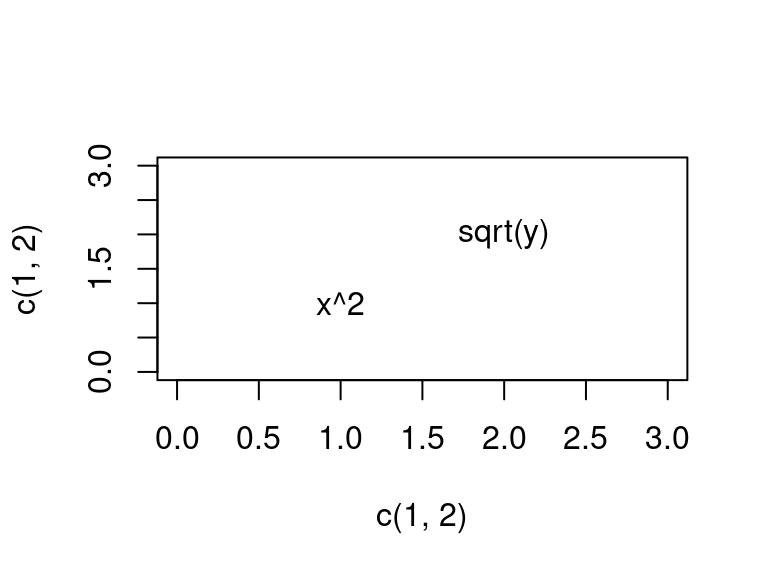

  

• For a {ggplot2} solution, I’ve found that I have to create a string that I then parse to an expression using parse = TRUE in geom_text():

  df <- data.frame(x = 1:2, y = 1:2, label = c("x^2", "sqrt(y)"))
  ggplot(data = df, mapping = aes(x = x, y = y, label = label)) +
    geom_text(parse = TRUE) +
    theme_bw()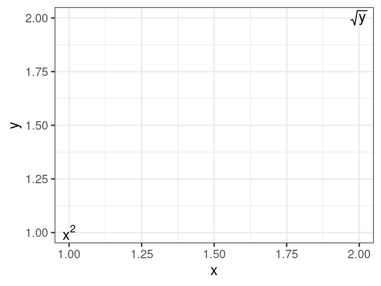

  

Application: Using the tidyverse in a function

• What if you want to create an awesome {ggplot2} function that allows the user to insert a data frame and output a simple scatterplot with red points. We will fill in the skeleton below.

  plot_red <- function(.data, var1, var2) {
  
  }

• If we want the user to not have to use strings for the variable names, then we need to capture those arguments

  plot_red <- function(.data, var1, var2) {
    var1 <- rlang::enexpr(var1)
    var2 <- rlang::enexpr(var2)
  }

• But if we were to just put var1 and var2 into {ggplot}, then {ggplot} would interpret that as trying to find a variable literally called var1 and var2 in .data. So we need to then unquote var1 and var2 in ggplot().

  plot_red <- function(.data, var1, var2) {
    var1 <- rlang::enexpr(var1)
    var2 <- rlang::enexpr(var2)
    ggplot(.data, aes(x = !!var1, y = !!var2)) +
      geom_point(col = "red")
  }

• This works now

  plot_red(.data = mtcars, var1 = wt, var2 = mpg)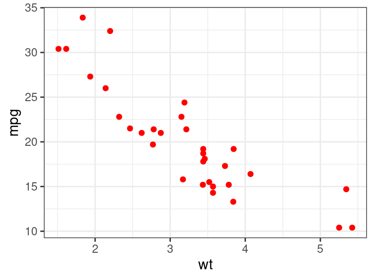

  

• Remember that the tidyverse mostly uses quoted arguments, not evaluated arguments, when choosing variable names. So this way of quoting and unquoting is common when coding using tidyverse functions.

• This also shows up in Shiny apps when you use varSelectInput().

Application: Using dplyr-Style Code on New Classes.

• In eval(), you can use a data.frame as the environment instead of an environment object. This is called data masking

  eval(expr = rlang::expr(mpg / wt), envir = mtcars)

  ##  [1]  8.015  7.304  9.828  6.656  5.436  5.231  4.006  7.649  7.238  5.581
  ## [11]  5.174  4.029  4.638  4.021  1.981  1.917  2.750 14.727 18.824 18.474
  ## [21]  8.722  4.403  4.425  3.464  4.993 14.109 12.150 20.093  4.984  7.112
  ## [31]  4.202  7.698

• This allows you to make tidyverse style functions without dependencies on the tidyverse.

• Some folks have explored this to the extreme.

• E.g. here is a variation of dplyr::filter() that only has a dependency on {rlang} (though, maybe not as safe as dplyr::filter() for some corner cases)

  #' @param .data A data.frame.
  #' @param e An expression.
  my_filter <- function(.data, e) {
    e <- rlang::enexpr(arg = e)
    .data[eval(expr = e, envir = .data), , drop = FALSE]
  }
  my_filter(mtcars, mpg > 30)

  ##                 mpg cyl disp  hp drat    wt  qsec vs am gear carb
  ## Fiat 128       32.4   4 78.7  66 4.08 2.200 19.47  1  1    4    1
  ## Honda Civic    30.4   4 75.7  52 4.93 1.615 18.52  1  1    4    2
  ## Toyota Corolla 33.9   4 71.1  65 4.22 1.835 19.90  1  1    4    1
  ## Lotus Europa   30.4   4 95.1 113 3.77 1.513 16.90  1  1    5    2

• Though, the {rlang} folks recommend you use quosures, not environments when doing data masking.

  #' @param .data A data.frame.
  #' @param e An expression.
  my_filter <- function(.data, e) {
    e <- rlang::enquo(arg = e)
    .data[rlang::eval_tidy(expr = e, data = .data), , drop = FALSE]
  }
  my_filter(mtcars, mpg > 30)

  ##                 mpg cyl disp  hp drat    wt  qsec vs am gear carb
  ## Fiat 128       32.4   4 78.7  66 4.08 2.200 19.47  1  1    4    1
  ## Honda Civic    30.4   4 75.7  52 4.93 1.615 18.52  1  1    4    2
  ## Toyota Corolla 33.9   4 71.1  65 4.22 1.835 19.90  1  1    4    1
  ## Lotus Europa   30.4   4 95.1 113 3.77 1.513 16.90  1  1    5    2

• You aren’t going to be using this filter function in real data analysis. But this style of metaprogramming is useful if you have an S3/S4 object and you want to provide {dplyr} style functionality.

• E.g., let’s create a class of two data frames where they are connected by a common key

  setClass(
    Class = "cdf", 
    slots = c(
      df1 = "data.frame", 
      df2 = "data.frame", 
      key = "character"
    ),
    prototype = list(
      df1 = data.frame(),
      df2 = data.frame(),
      key = character()
    )
  )
  
  setValidity(
    Class = "cdf", 
    method = function(object) {
      if (length(object@key) == 0 & ncol(object@df1) == 0 & ncol(object@df2) == 0) {
        return(TRUE)
      } else if (length(object@key) > 1) {
        return("key needs to be length 1")
      } else if (!(object@key %in% names(object@df1))) {
        return("key needs to be a column in df1")
      } else if (!(object@key %in% names(object@df1))) {
        return("key needs to be a column in df2")
      } else {
        return(TRUE)
      }
    }
  )

  ## Class "cdf" [in ".GlobalEnv"]
  ## 
  ## Slots:
  ##                                        
  ## Name:         df1        df2        key
  ## Class: data.frame data.frame  character

  setMethod(
    f = "show", 
    definition = function(object) {
      str(object@key)
      cat("\n")
      str(object@df1)
      cat("\n")
      str(object@df2)
    }
  )

• We can try this out on the nycflights13 dataset.

  library(nycflights13)
  mydf2 <- new(Class = "cdf", df1 = flights, df2 = planes, key = "tailnum")

• Let’s create a filter_df2() method that, when applied, will also remove all rows from df1 that have the keys that were removed from df2

  setGeneric(name = "filter_df2", def = function(obj, expr) standardGeneric("filter_df2"))

  ## [1] "filter_df2"

  setMethod(
    f = "filter_df2", 
    signature = "cdf", 
    definition = function(obj, expr) {
      expr <- rlang::enexpr(expr)
      logvec_df2 <- eval(expr = expr, envir = obj@df2)
      which_key <- obj@df2[[obj@key]][logvec_df2]
      logvec_df1 <- obj@df1[[obj@key]] %in% which_key
  
      obj@df1 <- obj@df1[logvec_df1, , drop = FALSE]
      obj@df2 <- obj@df2[logvec_df2, , drop = FALSE]
      return(obj)
    }
  )

• Let’s try it out

  filter_df2(obj = mydf2, tailnum == "N105UW")

  ##  chr "tailnum"
  ## 
  ## tibble [45 × 19] (S3: tbl_df/tbl/data.frame)
  ##  $ year          : int [1:45] 2013 2013 2013 2013 2013 2013 2013 2013 2013 2013 ...
  ##  $ month         : int [1:45] 10 10 10 11 11 11 11 12 12 12 ...
  ##  $ day           : int [1:45] 22 25 27 14 21 23 24 9 11 17 ...
  ##  $ dep_time      : int [1:45] 1312 1311 1543 1228 1549 1457 827 1159 1602 1152 ...
  ##  $ sched_dep_time: int [1:45] 1315 1315 1545 1200 1544 1500 825 1200 1544 1200 ...
  ##  $ dep_delay     : num [1:45] -3 -4 -2 28 5 -3 2 -1 18 -8 ...
  ##  $ arr_time      : int [1:45] 1458 1459 1747 1408 1752 1647 1029 1439 1848 1408 ...
  ##  $ sched_arr_time: int [1:45] 1505 1505 1751 1359 1750 1656 1029 1400 1750 1400 ...
  ##  $ arr_delay     : num [1:45] -7 -6 -4 9 2 -9 0 39 58 8 ...
  ##  $ carrier       : chr [1:45] "US" "US" "US" "US" ...
  ##  $ flight        : int [1:45] 2095 2095 1767 2069 1767 1834 2053 2069 1767 2069 ...
  ##  $ tailnum       : chr [1:45] "N105UW" "N105UW" "N105UW" "N105UW" ...
  ##  $ origin        : chr [1:45] "EWR" "EWR" "LGA" "JFK" ...
  ##  $ dest          : chr [1:45] "CLT" "CLT" "CLT" "CLT" ...
  ##  $ air_time      : num [1:45] 88 82 80 80 86 95 99 102 100 93 ...
  ##  $ distance      : num [1:45] 529 529 544 541 544 529 541 541 544 541 ...
  ##  $ hour          : num [1:45] 13 13 15 12 15 15 8 12 15 12 ...
  ##  $ minute        : num [1:45] 15 15 45 0 44 0 25 0 44 0 ...
  ##  $ time_hour     : POSIXct[1:45], format: "2013-10-22 13:00:00" "2013-10-25 13:00:00" ...
  ## 
  ## tibble [1 × 9] (S3: tbl_df/tbl/data.frame)
  ##  $ tailnum     : chr "N105UW"
  ##  $ year        : int 1999
  ##  $ type        : chr "Fixed wing multi engine"
  ##  $ manufacturer: chr "AIRBUS INDUSTRIE"
  ##  $ model       : chr "A320-214"
  ##  $ engines     : int 2
  ##  $ seats       : int 182
  ##  $ speed       : int NA
  ##  $ engine      : chr "Turbo-fan"

Exercises

1. Use rlang::call2() to create a call for table(x, y). Then remove the y component from that call to get table(x).

2. stats::numericDeriv() requires an expression and an environment. Calculate the derivative of log(x) / sin(x) evaluated at x = 2

3. You can calculate symbolic derivatives in R with D(), but you have to use expressions. Calculate the derivative of \(\sin(\cos(x + 1)^2)\). Then use that returned expression to evaluate the derivative at \(x =\) 1, 2, and 3.

4. Create your own version of stopifnot() called stop_if_not(). E.g.:

   stop_if_not(1 == 1, 2 > 1)
   stop_if_not(1 == 0)

   ## Error: ~1 == 0 is not TRUE

   stop_if_not(c(1,2,3) == 2)

   ## Error: ~c(1, 2, 3) == 2 is not length 1

   stop_if_not("potato")

   ## Error in stop_if_not("potato"): ~"potato" is not a predicate

   • Note: The {assertthat} package explores this idea to the extreme.

New Functions

• rlang::expr(): Create an expression (quote).
• rlang::enexpr(): Create an expression of an argument within a function (quote).
• base::eval(): Evaluate an expression.
• rlang::expr_text(): Convert an expression to text (deparse).
• rlang::call2(): Create a call from a function name and some expression arguments.
• !!: Unquote by evaluating single symbol.
• rlang::quo(): Create a quosure.
• rlang::enquo(): Create a quosure of an argument in within a function.
• rlang::eval_tidy(): Evaluate a quosure.

---

This work is licensed under a Creative Commons Attribution-NonCommercial 4.0 International License.