Tensors, or multidimensional arrays, are generalizations of vectors and matrices. Where a vector is a "line" of numbers and a matrix is a "rectangle" of numbers, a three-dimensional tensor is a "block" of numbers. Where a vector has one index and a matrix has two indices, a tensor may have three or more indices. Many modern data sets come in the form of tensors. Consider, for example, the multivariate longitudinal network data set on international trade from Hoff [2011]. This data set is a 4-dimensional tensor where the dimensions, or modes, are yearly change in log trade values in 2000 US dollars between 30 countries (modes 1 and 2) of 6 different commodities (mode 3) over 10 years (mode 4). A reasonable analysis for such data could proceed by fitting a model such as \(X = \Theta + E\), where \(X \in \mathbb{R}^{30 \times 30 \times 6 \times 10}\) is our data, \(\Theta\) is a low dimensional mean tensor, and \(E\) represents the additive residual variation about \(\Theta\). Most of the research in the field of tensor data analysis is in estimating \(\Theta\) through various "low rank" approximations of \(X\) (depending on one's generalization of rank to tensors), usually in terms of least squares. Much less work has been done on modeling the residual variation, \(E\). But such modeling is important for obtaining valid confidence intervals, improving prediction, and improving estimation of \(\Theta\) (via generalized least squares). To give a sense as to what kind of covariances may be present in such a data set, observe the following plot:
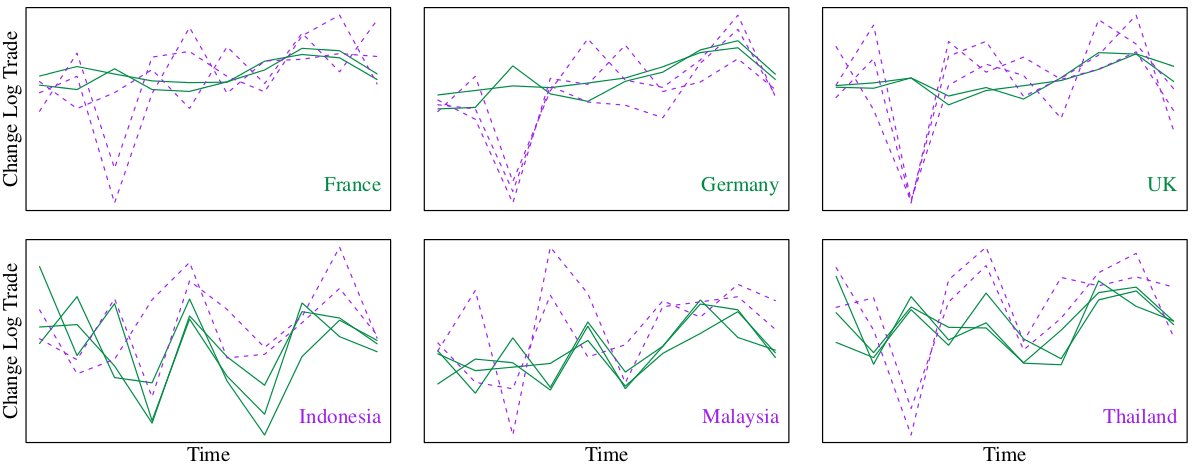
In the top left plot, for example, each line represents an exporting country, the \(x\)-axis is time in years, and the \(y\)-axis is the change in log-exports to France averaged over the commodity type. Some countries have similar exporting behavior (the solid green lines follow a similar trend). Some countries have similar importing behavior (the overall plots of Germany and France look similar). Adjacent years also seem to be negatively correlated (an increase in one year tends to be followed by a decrease in the next). One can also imagine that some commodities will vary in a similar pattern over time. All of this indicates that we should account for the dependencies along each dimension of this tensor when building a model.
One approach to modeling the residual variation in \(X\) would be to allow for unrestricted covariance between all the elements in \(E\) (except for positive definiteness constraints, of course). Although appealing, most tensor data sets have few replications --- for example, the trade data set above only has one replication. Even if we assumed that data from different years are independent, we would still be estimating a covariance matrix of dimension \(5400\) by \(5400\) as \(30 \times 30 \times 6 = 5400\), which is much greater than \(10\) (the size of the time dimension). It's apparent that we need to assume some covariance structure to obtain stable estimates.
One reasonable structure is found in the multilinear normal model, suggested by Hoff [2011]: \(X \overset{d}{=} \Theta + \sigma(\Psi_1,\ldots,\Psi_K) \cdot Z\), where \(\Psi_k \in \mathbb{R}^{p_k \times p_k}\) for \(k = 1,\ldots,K\), \(\sigma > 0\), \(Z \in \mathbb{R}^{p_1\times\cdots\times p_K}\) contains standard normal entries, and "\(\cdot\)" is "multilinear multiplication" or the "Tucker product" [Kolda, 2009]. If we were to "vectorize" \(X\), then the model is equivalently represented by
\[ \text{vec}(X) \sim N_{p}(\text{vec}(\Theta), \sigma^2\Psi_K\Psi_K^T \otimes \cdots \otimes \Psi_1\Psi_1^T), \]where "\(\otimes\)" is the Kronecker product and \(p = \prod_{k = 1}^K p_k\). That is, the multilinear normal model is the class of multivariate normal distributions with Kronecker structured covariance matrices. Not only is this model more parsimonious than fitting an unstructured covariance model (\(\sum_{k=1}^Kp_k(p_k+1)/2 - K + 1\) covariance parameters versus \((\prod_{k=1}^Kp_k)(\prod_{k=1}^K p_k + 1)/2\) covariance parameters), but the covariance parameters have a nice interpretation: If we "matricize" \(X\) along mode \(k\) to obtain \(X_{(k)} \in \mathbb{R}^{p_k \times \prod_{i\neq k}p_i}\), then the covariance of the columns of \(X_{(k)}\) can be shown to be proportional to \(\Psi_k\Psi_k^T\). That is, the covariance along each dimension may be represented by a single covariance matrix. With this model, we now need to find good estimators of the covariance parameters.
References
Hoff, P. D. (2011). Separable covariance arrays via the Tucker product, with applications to multivariate relational data. Bayesian Anal., 6(2), p. 179–196. doi:10.1214/11-BA606
Kolda, T. G., & Bader, B. W. (2009). Tensor decompositions and applications. SIAM review, 51(3), p. 455-500. doi:10.1137/07070111X