Introduction

R is a statistical programming language designed to analyze data.
This is not an R course. But you need to know some tools to summarize/plot/model data.
R is free, widely used, more generally applicable (beyond linear regression), and a useful tool for reproducibility. So this is what we will use.
Python would have been a good choice too, but you can learn that in the machine learning course (STAT 427/627).

Installation

Install here R : https://cran.r-project.org/
Install R Studio here: https://www.rstudio.com/
NOTE: R is a programming language. R Studio is an IDE, a program for interacting with programming language (specifically R in this case). Thus, on your resume, you should say that you know R, not R Studio.

Before we begin

I cannot teach you everything there is to know in R. When you know the name of a function, but don’t know the commands, use the help() function. For example, to learn more about log() type
```
help(log)
```
Alternatively, if you do not know the name of the function, you can Google the functionality you want. Googling coding solutions is a lot of what real data scientists do. Just append what you are Googling with “in R”. So, for example, “linear mixed effects models in R”.

R Basics

When you first open up R Studio, it should look something like this
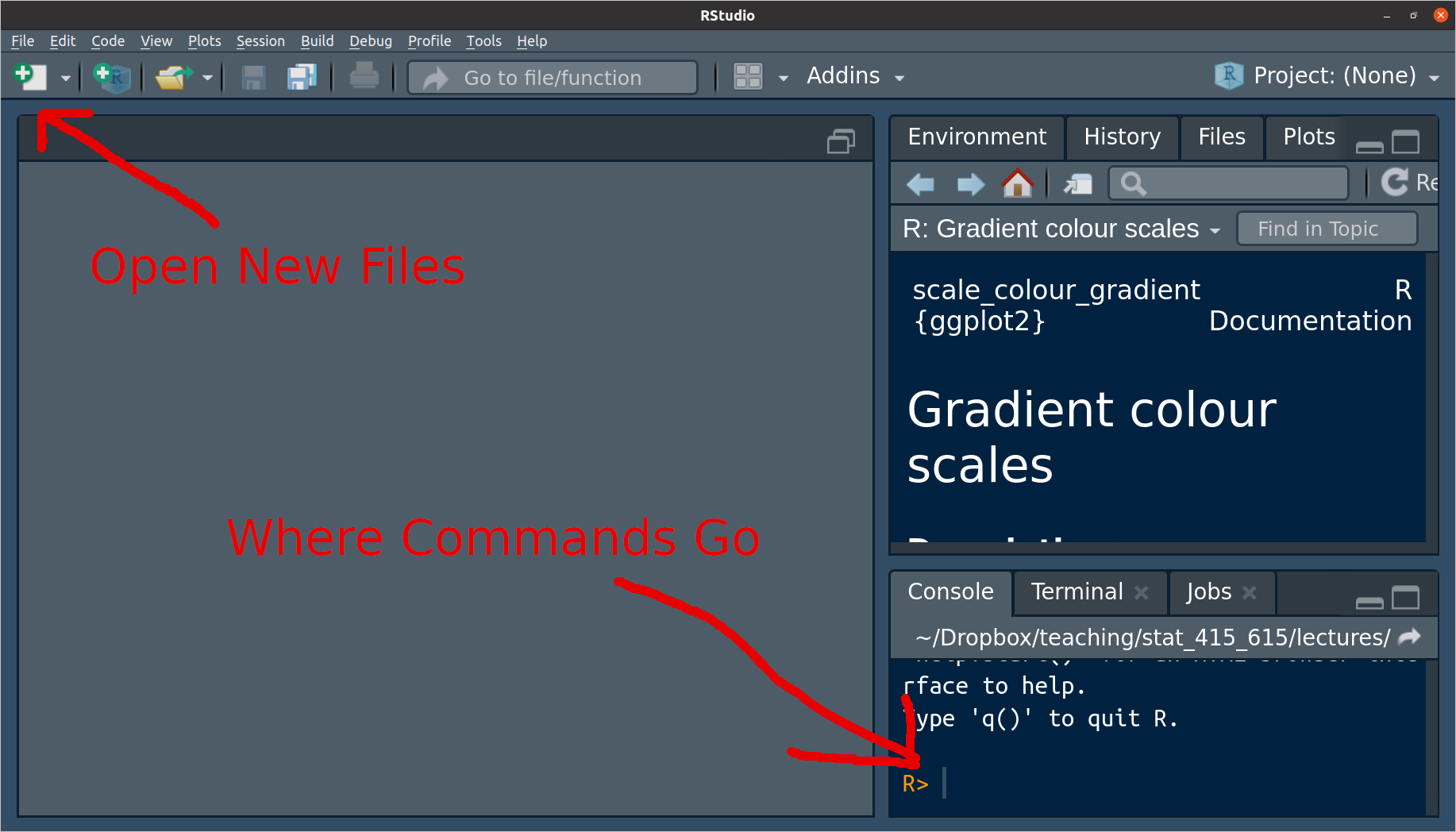
The area to the right of the carrot “>” is called a prompt. You insert commands into the prompt.
You can use R as a powerful calculator. Try typing some of the following into the command prompt:
```
3 * 7
9 / 3
4 + 6
3 - 9
(3 + 5) * 6
3 ^ 2
4 ^ 2
```
Exercise: What do you think the following will evaluate to? Try to guess before running it in R:
```
8 / 4 + 3 * 2 ^ 2
```
R consists of two things: variables and functions (computer scientists would probably disagree with this categorization).

Variables

A variable stores a value. You use the assignment operator “<-” to assign values to variables. For example, we can assign the value of 10 to the variable x.
```
x <- 10
```
- It is possible to use =, and I think there is nothing wrong with that. But for some reason the field has decided to only use <-, so you should too.
Whenever we use x later, it will use the value of 10
```
x
```
```
## [1] 10
```
This is useful because you can reuse this value over and over again:
```
y <- 0
x + y
x * y
x / y
x - y
```
To assign a “string” (a fancy way to say a word) to x, put the string in quotes. For example, we can assign the value of "Hello World" to x.
```
x <- "Hello World"
x
```
```
## [1] "Hello World"
```

Functions

Functions take objects (such as numbers or variables) as input and output new objects. Let’s look at a simple function that takes the log of a number:
```
log(x = 4, base = 2)
```
The inputs are called “arguments”. Generally, every function will be for the form:
```
function_name(arg1 = val1, arg2 = val2, ...)
```
If you do not specify the name of the argument, R will assume you are assigning in their order.
```
log(4, 2)
```
You can change the order of the arguments if you specify them.
```
log(base = 2, x = 4)
```
To see the list of all possible arguments of a function, use the help() function:
```
help(log)
```
In the help file, there are often default values for an argument. For example, the following indicates the the default value of base is exp(1).
```
log(x, base = exp(1))
```
This indicates that you can omit the base argument and R will assume that it should be exp(1).
```
log(x = 4, base = exp(1))
```
```
## [1] 1.386
```
```
log(x = 4)
```
```
## [1] 1.386
```
If an argument does not have a default, then it must be specified when calling a function.
Type this:
```
log(x = 4,
```
The “+” indicates that R is expecting more input (you forgot either a parentheses or a quotation mark). You can get back to the prompt by hitting the ESCAPE key.

Useful Functions

c() creates a vector (sequence of values)
```
y <- c(8, 1, 3, 4, 2)
y
```
```
## [1] 8 1 3 4 2
```

You can perform vectorized operations on these vectors

y + 2

## [1] 10  3  5  6  4

y / 2

## [1] 4.0 0.5 1.5 2.0 1.0

y - 2

## [1]  6 -1  1  2  0

exp(): Exponentiation. This is the inverse of log().
```
exp(10)
```
```
## [1] 22026
```
```
log(exp(10))
```
```
## [1] 10
```
mean(): The mean of a vector
```
mean(y)
```
```
## [1] 3.6
```
sd() The standard deviation of a vector
```
sd(y)
```
```
## [1] 2.702
```
sum(): Sum the values of a vector.
```
sum(y)
```
```
## [1] 18
```

seq(): Create a sequence of numbers

seq(from = 1, to = 10)

##  [1]  1  2  3  4  5  6  7  8  9 10

Exercise: What does the by argument do in seq()? Read the help file and modify it to 2 in the example code above.
head(): Show the first six values of an object.

R Packages

A package is a collection of functions that don’t come with R by default.
There are many many packages available. If you need to do any data analysis, there is probably an R package for it.
Using install.packages(), you can install packages that contain functions and datasets that are not available by default. Do this now with the tidyverse package:
```
install.packages("tidyverse")
```
You will only need to install a package once per computer. Once it is installed you can gain access to all of the functions and datasets in a package by using the library() function.
```
library(tidyverse)
```
You will need to run library() at the start of every R session if you want to use the functions in a package.
When I want to write the name of a function, I will write it like this().

Data Frames

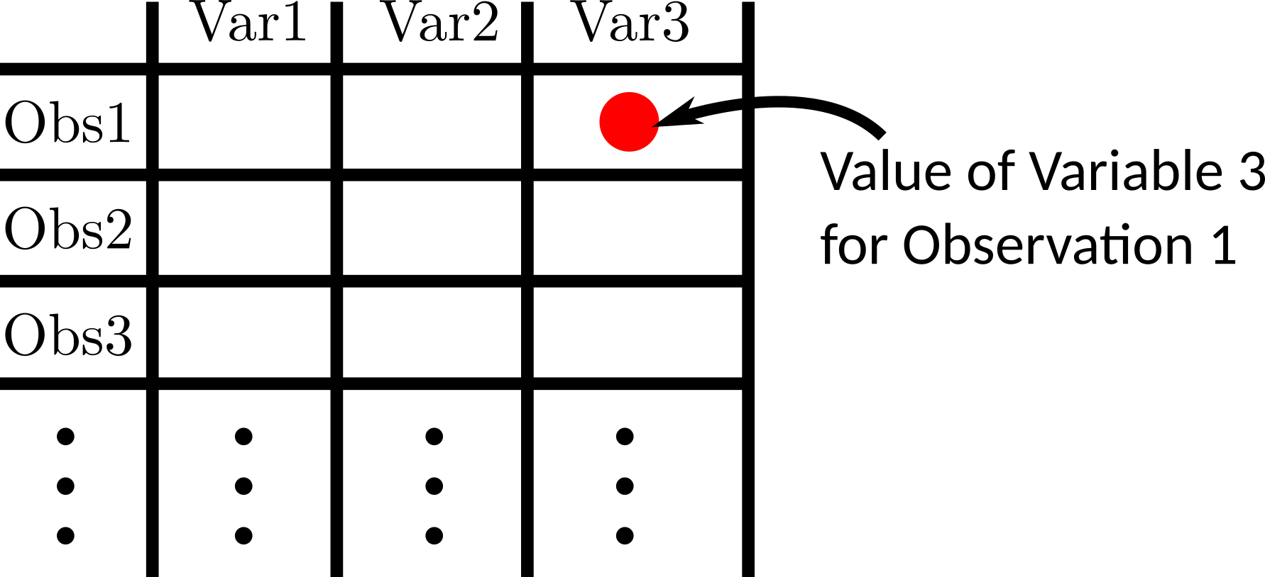
The fundamental unit object of data analysis is the data frame.
A data frame has variables in the columns, and observations in the rows.

R comes with a bunch of famous datasets in the form of a data frame. Such as the mtcars dataset.

data("mtcars")
mtcars

##                      mpg cyl  disp  hp drat    wt  qsec vs am gear carb
## Mazda RX4           21.0   6 160.0 110 3.90 2.620 16.46  0  1    4    4
## Mazda RX4 Wag       21.0   6 160.0 110 3.90 2.875 17.02  0  1    4    4
## Datsun 710          22.8   4 108.0  93 3.85 2.320 18.61  1  1    4    1
## Hornet 4 Drive      21.4   6 258.0 110 3.08 3.215 19.44  1  0    3    1
## Hornet Sportabout   18.7   8 360.0 175 3.15 3.440 17.02  0  0    3    2
## Valiant             18.1   6 225.0 105 2.76 3.460 20.22  1  0    3    1
## Duster 360          14.3   8 360.0 245 3.21 3.570 15.84  0  0    3    4
## Merc 240D           24.4   4 146.7  62 3.69 3.190 20.00  1  0    4    2
## Merc 230            22.8   4 140.8  95 3.92 3.150 22.90  1  0    4    2
## Merc 280            19.2   6 167.6 123 3.92 3.440 18.30  1  0    4    4
## Merc 280C           17.8   6 167.6 123 3.92 3.440 18.90  1  0    4    4
## Merc 450SE          16.4   8 275.8 180 3.07 4.070 17.40  0  0    3    3
## Merc 450SL          17.3   8 275.8 180 3.07 3.730 17.60  0  0    3    3
## Merc 450SLC         15.2   8 275.8 180 3.07 3.780 18.00  0  0    3    3
## Cadillac Fleetwood  10.4   8 472.0 205 2.93 5.250 17.98  0  0    3    4
## Lincoln Continental 10.4   8 460.0 215 3.00 5.424 17.82  0  0    3    4
## Chrysler Imperial   14.7   8 440.0 230 3.23 5.345 17.42  0  0    3    4
## Fiat 128            32.4   4  78.7  66 4.08 2.200 19.47  1  1    4    1
## Honda Civic         30.4   4  75.7  52 4.93 1.615 18.52  1  1    4    2
## Toyota Corolla      33.9   4  71.1  65 4.22 1.835 19.90  1  1    4    1
## Toyota Corona       21.5   4 120.1  97 3.70 2.465 20.01  1  0    3    1
## Dodge Challenger    15.5   8 318.0 150 2.76 3.520 16.87  0  0    3    2
## AMC Javelin         15.2   8 304.0 150 3.15 3.435 17.30  0  0    3    2
## Camaro Z28          13.3   8 350.0 245 3.73 3.840 15.41  0  0    3    4
## Pontiac Firebird    19.2   8 400.0 175 3.08 3.845 17.05  0  0    3    2
## Fiat X1-9           27.3   4  79.0  66 4.08 1.935 18.90  1  1    4    1
## Porsche 914-2       26.0   4 120.3  91 4.43 2.140 16.70  0  1    5    2
## Lotus Europa        30.4   4  95.1 113 3.77 1.513 16.90  1  1    5    2
## Ford Pantera L      15.8   8 351.0 264 4.22 3.170 14.50  0  1    5    4
## Ferrari Dino        19.7   6 145.0 175 3.62 2.770 15.50  0  1    5    6
## Maserati Bora       15.0   8 301.0 335 3.54 3.570 14.60  0  1    5    8
## Volvo 142E          21.4   4 121.0 109 4.11 2.780 18.60  1  1    4    2

You can extract individual variables from a data frame using $

mtcars$mpg

##  [1] 21.0 21.0 22.8 21.4 18.7 18.1 14.3 24.4 22.8 19.2 17.8 16.4 17.3 15.2 10.4
## [16] 10.4 14.7 32.4 30.4 33.9 21.5 15.5 15.2 13.3 19.2 27.3 26.0 30.4 15.8 19.7
## [31] 15.0 21.4

You can explore these in a spreadsheet format using View() (note the capital “V”).
```
View(mtcars)
```

Reading in Data Frames

Most datasets will nead to be loaded into R. To do so, we will use the {readr} package.
```
library(readr)
```
The only function I will require you to know from this package is read_csv(), which loads in data from a CSV file (“Comma-separated values”), a very popular format for storing data.
If you have the CSV file somewhere on your computer, then specify the path from the current working directory, and assign the data frame to a variable.
For other file formats, you need to use other functions, such as read_tsv(), read_table(), read_fwf(), etc. I will try to make sure read_csv() works for all datasets in this course.

I will typicaly post course datasets at https://dcgerard.github.io/stat_415_615/data.html. You can load those data into R by pasting their URL’s into read_csv().

copiers <- read_csv("https://dcgerard.github.io/stat_415_615/data/copiers.csv")

## Rows: 45 Columns: 3
## ── Column specification ────────────────────────────────────────────────────────
## Delimiter: ","
## chr (1): model
## dbl (2): minutes, copiers
## 
## ℹ Use `spec()` to retrieve the full column specification for this data.
## ℹ Specify the column types or set `show_col_types = FALSE` to quiet this message.

head(copiers)

## # A tibble: 6 × 3
##   minutes copiers model
##     <dbl>   <dbl> <chr>
## 1      20       2 S    
## 2      60       4 L    
## 3      46       3 L    
## 4      41       2 L    
## 5      12       1 L    
## 6     137      10 L

Exercise: Load in the County Demographic Information data into R and print out the first six rows.

Basic Data Frame Manipulations

You will need to know just a few data frame manipulations, which we will perform using the {dplyr} package.
```
library(dplyr)
```
The first argument for {dplyr} functions is always the data frame you are modifying. The following arguments typically involve the columns of that data frame.

Use the mutate() function from the {dplyr} package to make variable transformations.

mtcars <- mutate(mtcars, kpg = mpg * 1.61)
head(mtcars)

##                    mpg cyl disp  hp drat    wt  qsec vs am gear carb   kpg
## Mazda RX4         21.0   6  160 110 3.90 2.620 16.46  0  1    4    4 33.81
## Mazda RX4 Wag     21.0   6  160 110 3.90 2.875 17.02  0  1    4    4 33.81
## Datsun 710        22.8   4  108  93 3.85 2.320 18.61  1  1    4    1 36.71
## Hornet 4 Drive    21.4   6  258 110 3.08 3.215 19.44  1  0    3    1 34.45
## Hornet Sportabout 18.7   8  360 175 3.15 3.440 17.02  0  0    3    2 30.11
## Valiant           18.1   6  225 105 2.76 3.460 20.22  1  0    3    1 29.14

Use glimpse() to get a brief look at the data frame.

glimpse(mtcars)

## Rows: 32
## Columns: 12
## $ mpg  <dbl> 21.0, 21.0, 22.8, 21.4, 18.7, 18.1, 14.3, 24.4, 22.8, 19.2, 17.8,…
## $ cyl  <dbl> 6, 6, 4, 6, 8, 6, 8, 4, 4, 6, 6, 8, 8, 8, 8, 8, 8, 4, 4, 4, 4, 8,…
## $ disp <dbl> 160.0, 160.0, 108.0, 258.0, 360.0, 225.0, 360.0, 146.7, 140.8, 16…
## $ hp   <dbl> 110, 110, 93, 110, 175, 105, 245, 62, 95, 123, 123, 180, 180, 180…
## $ drat <dbl> 3.90, 3.90, 3.85, 3.08, 3.15, 2.76, 3.21, 3.69, 3.92, 3.92, 3.92,…
## $ wt   <dbl> 2.620, 2.875, 2.320, 3.215, 3.440, 3.460, 3.570, 3.190, 3.150, 3.…
## $ qsec <dbl> 16.46, 17.02, 18.61, 19.44, 17.02, 20.22, 15.84, 20.00, 22.90, 18…
## $ vs   <dbl> 0, 0, 1, 1, 0, 1, 0, 1, 1, 1, 1, 0, 0, 0, 0, 0, 0, 1, 1, 1, 1, 0,…
## $ am   <dbl> 1, 1, 1, 0, 0, 0, 0, 0, 0, 0, 0, 0, 0, 0, 0, 0, 0, 1, 1, 1, 0, 0,…
## $ gear <dbl> 4, 4, 4, 3, 3, 3, 3, 4, 4, 4, 4, 3, 3, 3, 3, 3, 3, 4, 4, 4, 3, 3,…
## $ carb <dbl> 4, 4, 1, 1, 2, 1, 4, 2, 2, 4, 4, 3, 3, 3, 4, 4, 4, 1, 2, 1, 1, 2,…
## $ kpg  <dbl> 33.81, 33.81, 36.71, 34.45, 30.11, 29.14, 23.02, 39.28, 36.71, 30…

Use View() to see a spreadsheet of the data frame (never put this in an R Markdown file). Note the capital “V”.
```
View(mtcars)
```

Use rename() to rename variables.

mtcars <- rename(mtcars, auto_man = am)
head(mtcars)

##                    mpg cyl disp  hp drat    wt  qsec vs auto_man gear carb
## Mazda RX4         21.0   6  160 110 3.90 2.620 16.46  0        1    4    4
## Mazda RX4 Wag     21.0   6  160 110 3.90 2.875 17.02  0        1    4    4
## Datsun 710        22.8   4  108  93 3.85 2.320 18.61  1        1    4    1
## Hornet 4 Drive    21.4   6  258 110 3.08 3.215 19.44  1        0    3    1
## Hornet Sportabout 18.7   8  360 175 3.15 3.440 17.02  0        0    3    2
## Valiant           18.1   6  225 105 2.76 3.460 20.22  1        0    3    1
##                     kpg
## Mazda RX4         33.81
## Mazda RX4 Wag     33.81
## Datsun 710        36.71
## Hornet 4 Drive    34.45
## Hornet Sportabout 30.11
## Valiant           29.14

Use filter() to remove rows.

Use == to select rows based on equality
Use < and > to select rows based on inequality
Use <= and >= to select rows based on inequality/equality.

filter(mtcars, auto_man == 1)

##                 mpg cyl  disp  hp drat    wt  qsec vs auto_man gear carb   kpg
## Mazda RX4      21.0   6 160.0 110 3.90 2.620 16.46  0        1    4    4 33.81
## Mazda RX4 Wag  21.0   6 160.0 110 3.90 2.875 17.02  0        1    4    4 33.81
## Datsun 710     22.8   4 108.0  93 3.85 2.320 18.61  1        1    4    1 36.71
## Fiat 128       32.4   4  78.7  66 4.08 2.200 19.47  1        1    4    1 52.16
## Honda Civic    30.4   4  75.7  52 4.93 1.615 18.52  1        1    4    2 48.94
## Toyota Corolla 33.9   4  71.1  65 4.22 1.835 19.90  1        1    4    1 54.58
## Fiat X1-9      27.3   4  79.0  66 4.08 1.935 18.90  1        1    4    1 43.95
## Porsche 914-2  26.0   4 120.3  91 4.43 2.140 16.70  0        1    5    2 41.86
## Lotus Europa   30.4   4  95.1 113 3.77 1.513 16.90  1        1    5    2 48.94
## Ford Pantera L 15.8   8 351.0 264 4.22 3.170 14.50  0        1    5    4 25.44
## Ferrari Dino   19.7   6 145.0 175 3.62 2.770 15.50  0        1    5    6 31.72
## Maserati Bora  15.0   8 301.0 335 3.54 3.570 14.60  0        1    5    8 24.15
## Volvo 142E     21.4   4 121.0 109 4.11 2.780 18.60  1        1    4    2 34.45

filter(mtcars, mpg < 15)

##                      mpg cyl disp  hp drat    wt  qsec vs auto_man gear carb
## Duster 360          14.3   8  360 245 3.21 3.570 15.84  0        0    3    4
## Cadillac Fleetwood  10.4   8  472 205 2.93 5.250 17.98  0        0    3    4
## Lincoln Continental 10.4   8  460 215 3.00 5.424 17.82  0        0    3    4
## Chrysler Imperial   14.7   8  440 230 3.23 5.345 17.42  0        0    3    4
## Camaro Z28          13.3   8  350 245 3.73 3.840 15.41  0        0    3    4
##                       kpg
## Duster 360          23.02
## Cadillac Fleetwood  16.74
## Lincoln Continental 16.74
## Chrysler Imperial   23.67
## Camaro Z28          21.41

Exercise: Calculate the log-displacement, add this to the mtcars data frame.
Exercise: Filter out cars with only one carborator (keep cars with more than 1 carborator).
Exercise: Rename the hp variable to horse.

Summary

Here is the list of basic R stuff I expect you to know off the top of your head. We will add to this list throughout the semester.

help(): Open help file.
install.packages(): Install an external R package. Do this once per computer for each package.
library(): Load the functions of an external R package so you can use them. Do this each time you start up R for each package.
<-: Variable assignment.
+, -, /, *: Arithmetic operations.
^: Powers.
sqrt(): Square root.
log(): Log (base e).
$: Extracting a variable from a data frame.
View(): Look at a spreadsheet of data.
head(): See first six elements.
From {readr}:
- read_csv(): Loading in tabular data.
From {dplyr}:
- glimpse(): Look at a data frame.
- mutate(): Variable transformation.
- rename(): Variable renaming.
- filter(): Select rows based on variable values.
From {ggplot2} (see 01_ggplot).
- ggplot2(): Set a dataset and aesthetic map.
- geom_point(): Make a scatterplot.
- geom_histogram(): Make a histogram.
- geom_bar(): Make a bar plot.
- geom_boxplot(): Make a box plot.
- geom_smooth(): Add a smoother.

Introduction to R

David Gerard

2022-12-01