Learning Objectives

Minimum mathematics required to complete this course.
Summations/averages
Equations for lines
Logarithms/exponentials
Chapter 3 of ROS

Motivation

Mathematics are the building blocks of linear regression.
You must be proficient with linear equations and summations to implement and understand linear models.
Log/exponential transformations are important for the practice and interpretation of many types of linear models.
Here, we will provide a brief mathematical review.

Weighted Averages

Consider the following data on USA, Mexico, and Canada:

Label Population $N_j$ Average Age $\bar{y}_j$

USA 310 Million 36.8

Mexico 112 Million 26.7

Canada 34 Million 40.7
What is the average age for these three countries?
Proportion USA: $\frac{310}{310 + 112 + 34} = 0.68$.
Proportion Mexico: $\frac{112}{310 + 112 + 34} = 0.25$.
Proportion Canada: $\frac{34}{310 + 112 + 34} = 0.07$.
So the USA contributes 68% of the population, mexico contributes 25% of the population, and Canada contributes 7% of the population. To find the overall average age, we calculate:

Label	Population \(N_j\)	Average Age \(\bar{y}_j\)
USA	310 Million	36.8
Mexico	112 Million	26.7
Canada	34 Million	40.7

\[ 0.68 \times 36.8 + 0.25 \times 26.7 + 0.07 \times 40.7 = 34.6 \]

We can equivalently write this as

\[ \frac{310 \times 36.8 + 112 \times 26.7 + 34 \times 40.7}{310 + 112 + 34} = \frac{310}{456}\times 36.8 + \frac{112}{456}\times 26.7 + \frac{34}{456}\times 40.7 \]

The proportions 0.68, 0.25, and 0.07 are called the weights. When the weights sum to one, the overall sumation is called a weighted average.
In summation notation (using the capital-sigma), we would write:

\[\begin{align} \text{weighted average} &= \sum_{j=1}^n w_j y_j\\ &= w_1y_1 + w_2y_2 + \cdots w_ny_n \end{align}\]

where $w_j$ is the $j$th weight and $y_j$ is the $j$th value.
What would be an “unweighted” average? This is where each $w_j = \frac{1}{n}$ since

\[\begin{align} \sum_{j=1}^n w_j y_j &= \sum_{j=1}^n \frac{1}{n} y_j\\ &= \frac{1}{n}y_1 + \frac{1}{n}y_2 + \cdots + \frac{1}{n}y_n\\ &= \frac{1}{n}(y_1 +y_2 + \cdots + y_n)\\ &= \frac{1}{n}\sum_{j=1}^n y_j\\ &= \bar{y} \end{align}\]
Properties of summations:
- $\sum_{i=1}^n c a_i = c\sum_{i=1}^na_i$
- $\sum_{i=1}^n a_i + \sum_{i=1}^nb_i = \sum_{i=1}^n(a_i + b_i)$
Exercise: 51% of Americans are female while 49% of Americans are male. 79% of teachers are female while 21% of teachers are male. Female teachers make on average $45,865, while male teachers make on average $49,207. What is the average salary for all teachers?
Exercise: What is $\sum_{i=0}^4 i$?
Exercise: Prove that it is not generally true that $\left(\sum_{i=1}^n y_i\right)^2 = \sum_{i=1}^n y_i^2$ (hint: provide a counterexample).

Products

We use capital-pi notation to represent product.

\[ \prod_{i=1}^n a_i = a_1 \times a_2 \times \cdots \times a_n \]

Lines

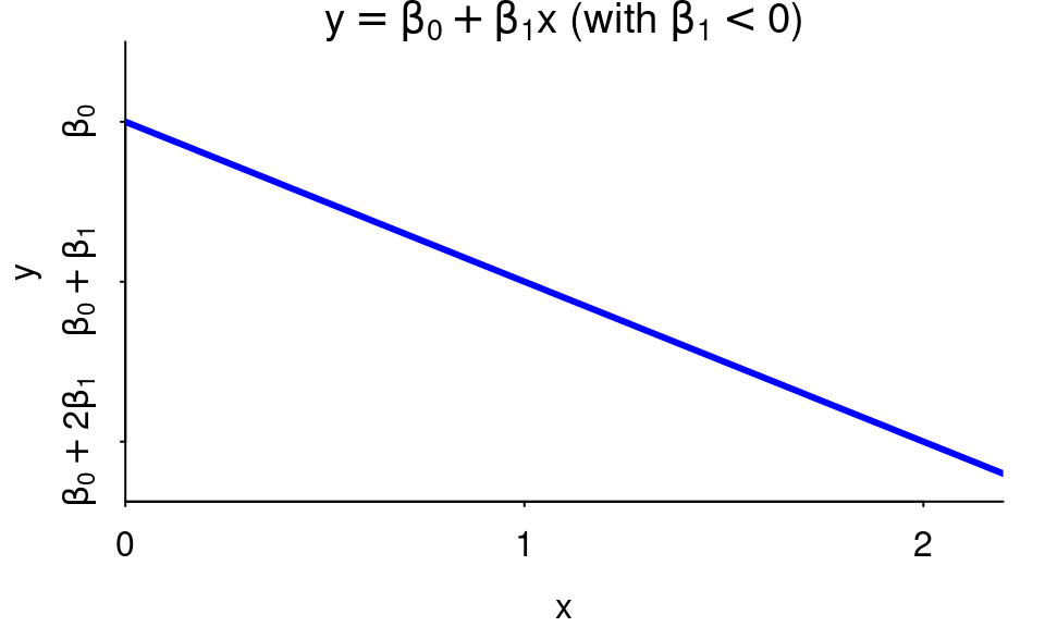
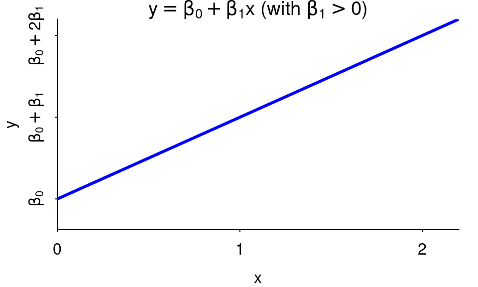
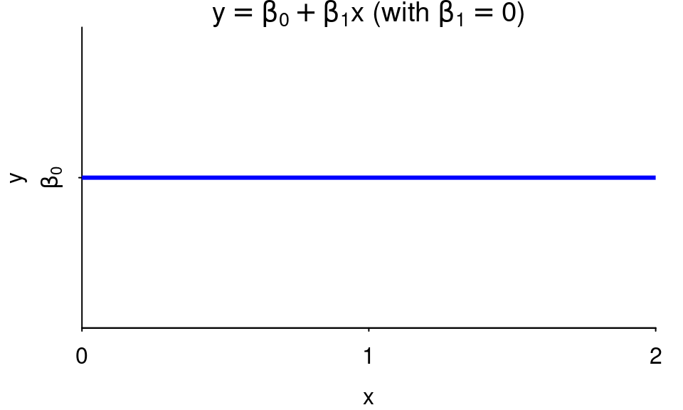
All lines are of the form \[ y = \beta_0 + \beta_1 x \]
$\beta_1$ is the slope, the amount $y$ is larger by when $x$ is 1 unit larger.
When $\beta_1$ is negative, the line slopes down.
When $\beta_1$ is positive, the line slopes up.
When $\beta_1$ is 0, the line is horizontal. In this case, $y$ is the same for every value of $x$ (in other words, $x$ does not affect $y$).

Example: The progression of mile world records during the 20th century is well approximated by the line $y = 1007 - 0.393x$

library(readr)
library(ggplot2)
mile <- read_csv("https://dcgerard.github.io/stat_415_615/data/mile.csv")
ggplot(data = mile, mapping = aes(x = year, y = seconds)) +
  geom_point() +
  geom_abline(slope = -0.393, intercept = 1007, lty = 2, col = 2)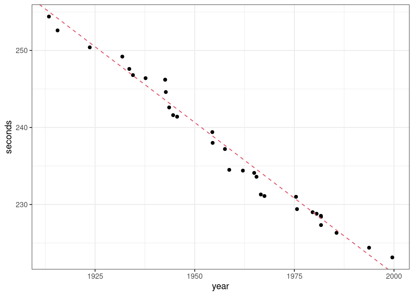

The world record in 1950 was about \[ y = 1007 - 0.393 * 1950 = 240.6 \text{ seconds}, \] which is actually between the two world record values of 241.4 seconds in 1946 and 239.4 seconds in 1954.
Interpretation of $\beta_0$: Can we interpret 1007 seconds (16.8 minutes) as the approximate world record in ancient times? No! Our data are only from 1913 to 1999, so this is an obviously improper extrapolation. It is just the $y$-intercept, with no other interpretation.
Interpretation of $\beta_1$: Each year, on average, the world record is 0.393 seconds lower.
Do not say “the world record decreases by about 0.393 seconds each year” as this creates an implicit causal connection.
Exercise: Year versus maximum life expectancy (where maximum was taken over country) is well approximated by the line $y = -296 + 0.189 x$.
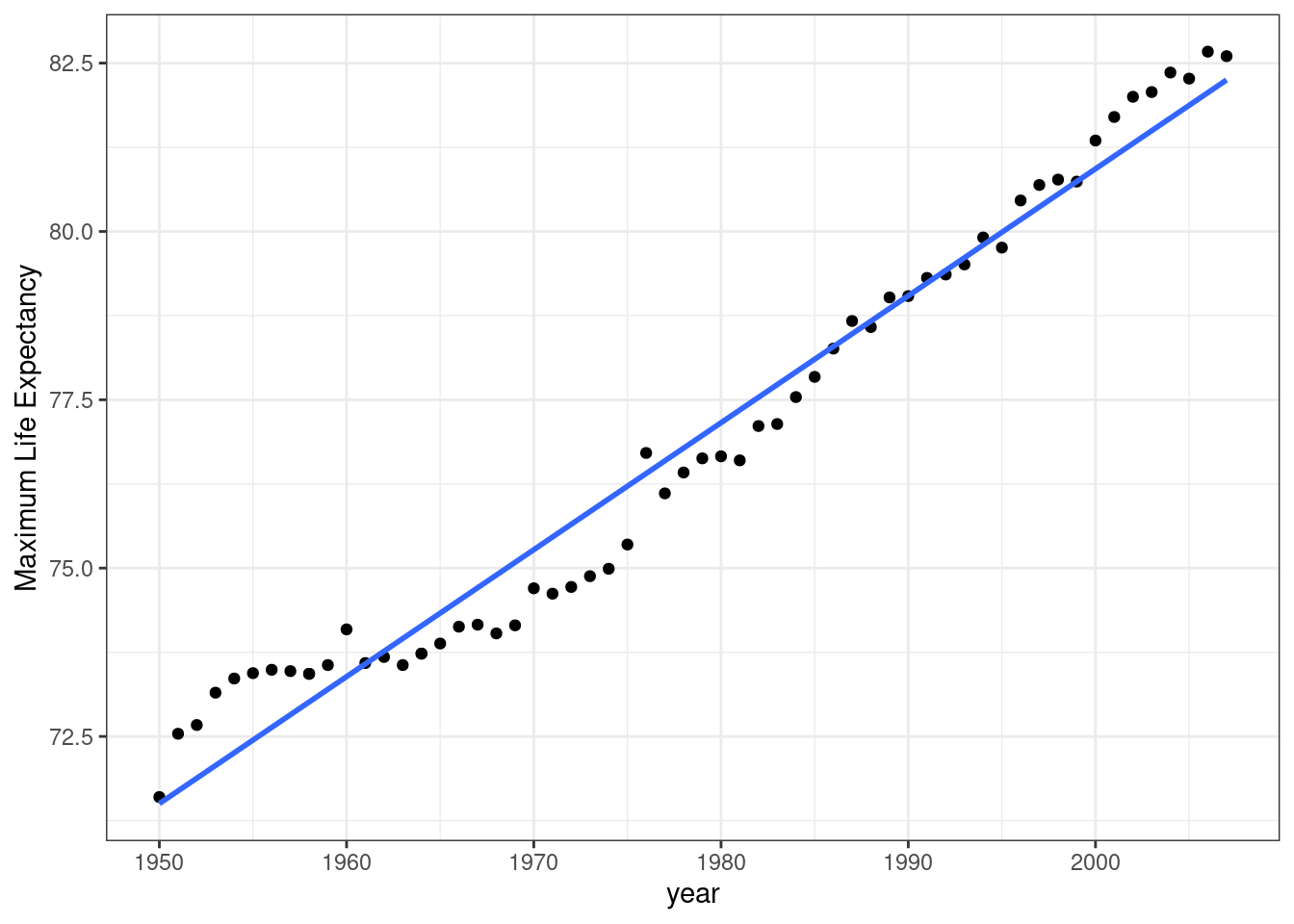
1. What is the expected life expectancy in 1990?
2. Interpret -296
3. Interpret 0.189

Additive/Multiplicative Comparisons

This semester, we will spend a lot of time talking about differences in one variable associated with differences in another variable.
We need to know how to properly speak about “differences”, or “numerical comparisons”.
Suppose car $A$ has a gas mileage of 30 mpg, and car $B$ has a gas mileage of 20 mpg. Then obviously car $A$ has 10 mpg better gas mileage. This is called an additive comparison since we can write it as $A + -B = 10$.
- Wikipedia calls this an “absolute difference”.
We can also describe this comparison as multiplicative. Here are some common ways to describe multiplicative comparisons.
- Wikipedia calls this a “relative difference”
$A$ has 50 percent more gas mileage than $B$.
- $A = B(1 + 0.5) = B + 0.5B = B + 50\% B$
- Thus, $A$ is $B$ plus 50 percent of $B$’s value. This is why we say “50 percent more”.
- In general, $A$ is $\frac{A - B}{B} \times 100\%$ larger than $B$
$B$ has 66.7 percent the value of $A$.
- This is since $B / A = 2/3 \approx 0.667 = 66.7\%$.
- In general, $B$ has $\frac{B}{A}\times 100\%$ the value of $A$.
$A$ has 150 percent the value of $B$.
- This is since $A / B = 3/2 = 1.5 = 150\%$
- In general, $A$ has $\frac{A}{B}\times 100\%$ the value of $B$.
$B$ has 33.3 percent less gas mileage than $A$.
- $B = A(1 - 1/3) = A - (1/3)A \approx A - 0.333A = A - 33.3\%A$
- Thus, $B$ is $A$ minus 33.3 percent of $A$’s value. This is why we say “33.3 percent less”.
- In general, $B$ is $\frac{A-B}{A}\times 100\%$ smaller than $A$.
Exercise: Suppose John makes $40,000 a year and Alina makes $50,000 a year. Provide four different ways to describe the multiplicative comparison between John’s and Alina’s salaries.
Sometimes we have additive comparsons for a variable whose scale is percent.
For example, candidate $A$ won 40% of the vote, and candidate $B$ won 30% of the vote.
If we want to describe the additive comparison between these two candidates, we cannot say “percent” because that would imply a mulitiplicative comparison.
To describe additive comparisons of a variable whose units are percent, we say percentage point.
Thus, candidate $A$’s vote share is 10 percentage points higher than candidate $B$’s.
We can still describe multiplicative comparisons for these variables. E.g. Candidate $A$’s vote share is 33.3 percent higher than candidate $B$’s.

Logarithms and Exponentials

Often, we consider linear relationships on the log-scale. So we need to know something about logarithms and exponentials.
Let’s start with exponentials: \[ \exp(x) = e^x = \underbrace{e \times \dots \times e}_{x\, \textrm{times}} \].
```
## Define e
e <- exp(1)
e
```
```
## [1] 2.718
```
```
## show exp(3) == e * e * e
exp(3) 
```
```
## [1] 20.09
```
```
e * e * e
```
```
## [1] 20.09
```
Recall that $e$ is Euler’s number, which is about 2.7183.
The last equality in the above equation for exp() only follows if $x$ is positive integer, but exponentiation can be extended to any real number.
```
exp(1.414)
```
```
## [1] 4.112
```
$\log(x)$ is the natural logarithm of $x$ (not base 10). This is the inverse of exponentiation \[ \log(\exp(x)) = \exp(\log(x)) = x \]

You can verify this in R

exp(log(31))

## [1] 31

log(exp(31))

## [1] 31

You can also interpret $\log(x)$ as the number of times you have to divide $x$ by $e$ to obtain 1. For example, since you would have to divide $e^4$ by $e$ 4 times to get 1 ($1 = \frac{e^4}{e \times e \times e \times e}$), we have that $\log(e^4) = 4$.
A useful property of logs/exponents is how it can convert multiplication to summation and vice versa.
- $\exp(a + b) = \exp(a)\exp(b)$.
- $\log(ab) = \log(a) + \log(b)$.
Why do we care about exponentials and logarithms? Because many relationships in the real world follow exponential or power laws.

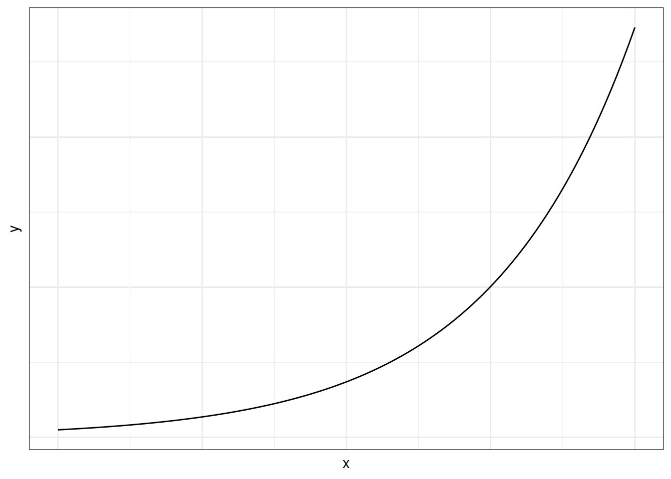
Exponential growth/decline

$\log(y) = \beta_0 + \beta_1 x$ represents exponential growth if $\beta_1 > 0$ and exponential decline if $\beta_1 < 0$.
Exponentiating both sides, we get \[ y = e^{\beta_0}e^{\beta_1 x} \]
Exponential growth:
Exponential decline:
$e^{\beta_0}$ is the value of $y$ when $x = 0$
$\beta_1$ determines the rate of growth or decline.
A 1-unit difference in $x$ corresponds to a multiplicative factor of $e^{\beta_1}$ in $y$. (you multiply the old $y$ value by $e^{\beta_1}$ to figure out the new $y$ value when you have an $x$ value that is 1 larger).
This follows from: \[\begin{align} y_{old} &= e^{\beta_0}e^{\beta_1 x}\\ y_{new} &= e^{\beta_0}e^{\beta_1 (x + 1)}\\ &= e^{\beta_0}e^{\beta_1 x + \beta_1}\\ &= e^{\beta_0}e^{\beta_1 x} e^{\beta_1}\\ &= y_{old}e^{\beta_1} \end{align}\]

Example: The early growth of COVID-19 in DC looked exponential:

dc <- read_csv("https://dcgerard.github.io/stat_415_615/data/dccovid.csv")
dc <- select(dc, day, positives)
dc <- filter(dc, day <= "2020-04-01", day >= "2020-03-11") 
ggplot(data = dc, mapping = aes(x = day, y = positives)) +
  geom_point()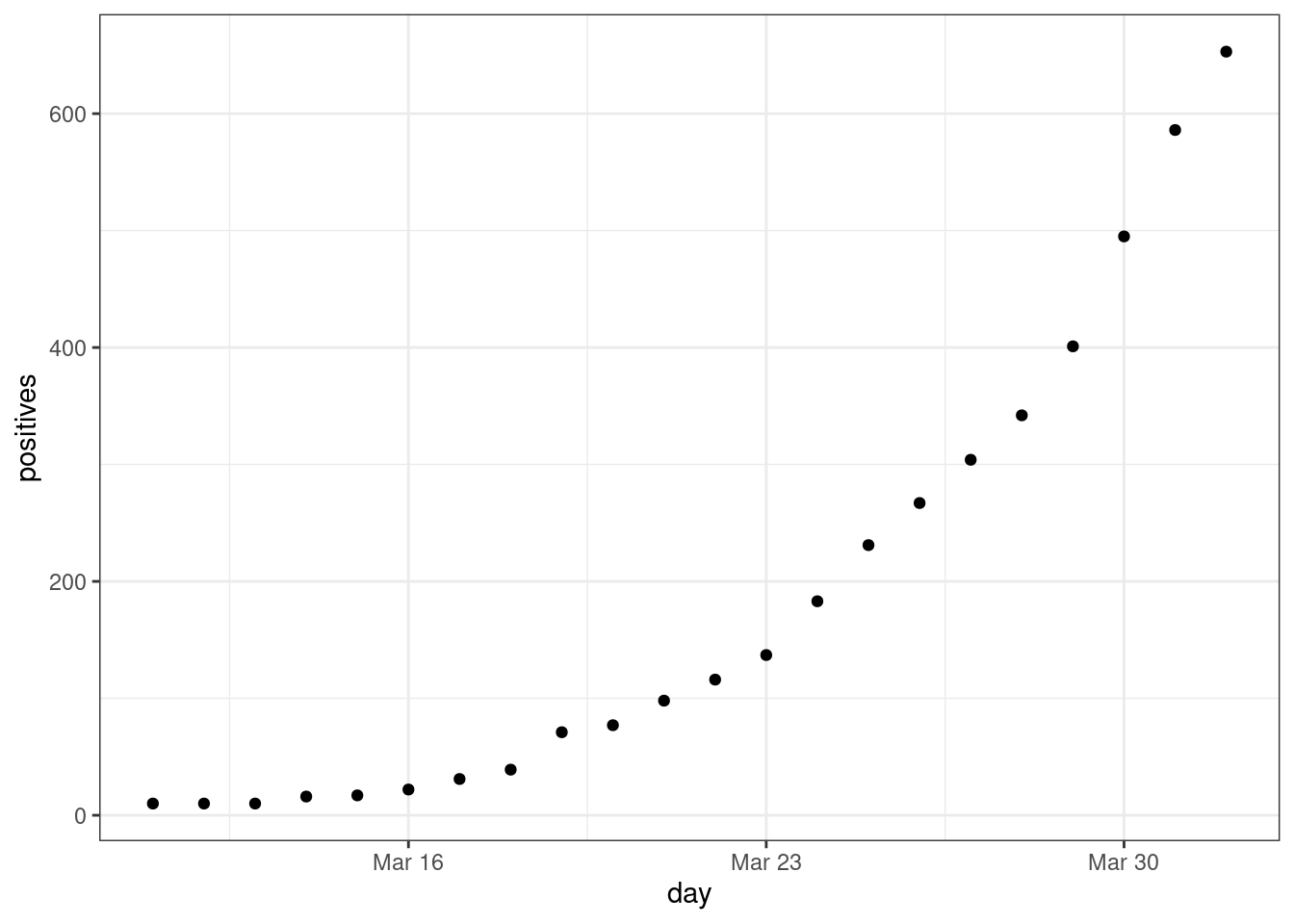

We determine if an exponential growth model is appropriate by seeing if day versus log-positives is approximately linear:

dc <- mutate(dc, 
             lpos = log(positives),
             daysin = as.numeric(day) - as.numeric(day[[1]]))
ggplot(data = dc, mapping = aes(x = daysin, y = lpos)) +
  geom_point()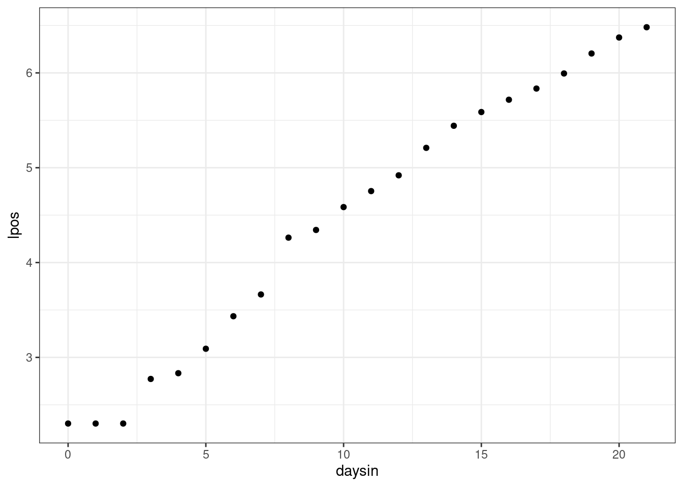

A curve that fits this growth well is $y = 8.8815e^{0.218x}$.

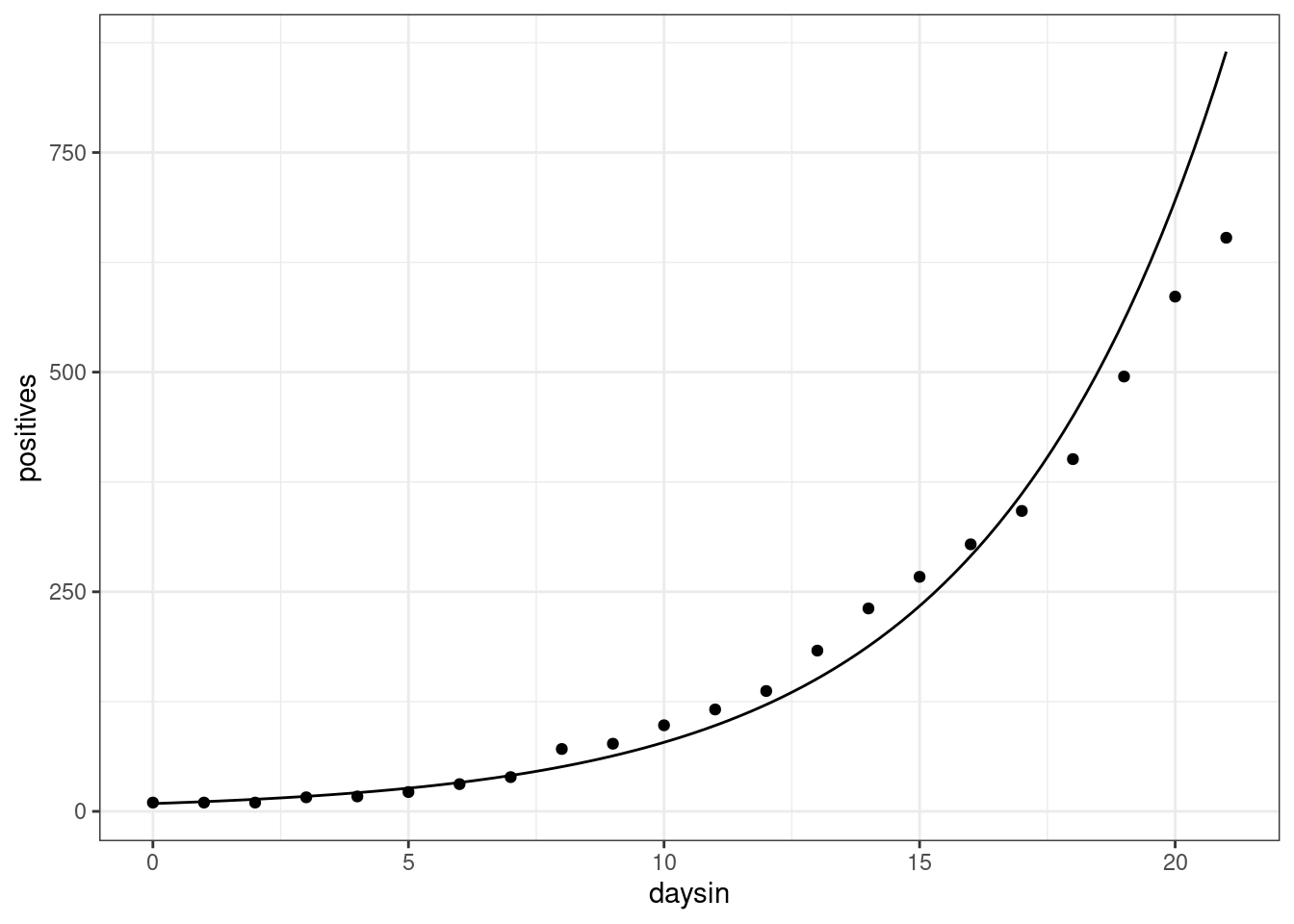
So that means that early on in the pandemic, each day positive tests were multiplicatively larger by about $e^{\beta_1} = e^{0.218} = 1.2436$. Or, about a 24% larger each day.

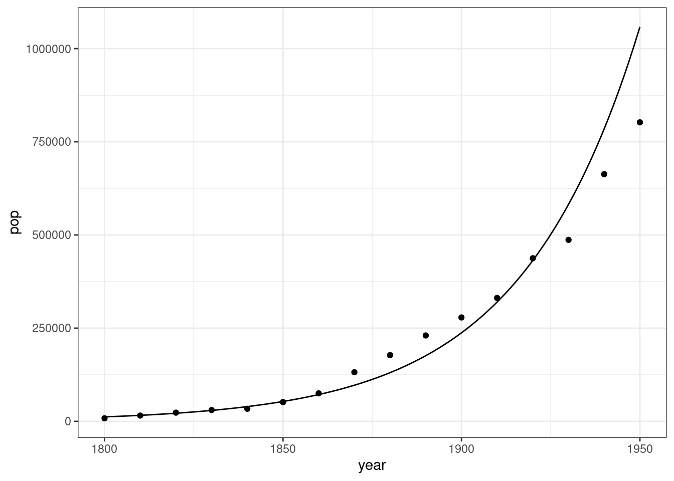
Exercise: Consider the population growth of DC from 1800 to 1950, taken from Wikipedia.

dcpop <- tribble(~year,   ~pop,
                 1800L,   8144,
                 1810L,  15471,
                 1820L,  23336,
                 1830L,  30261,
                 1840L,  33745,
                 1850L,  51687,
                 1860L,  75080,
                 1870L, 131700,
                 1880L, 177624,
                 1890L, 230392,
                 1900L, 278718,
                 1910L, 331069,
                 1920L, 437571,
                 1930L, 486869,
                 1940L, 663091,
                 1950L, 802178)
ggplot(data = dcpop, mapping = aes(x = year, y = pop)) +
  geom_point()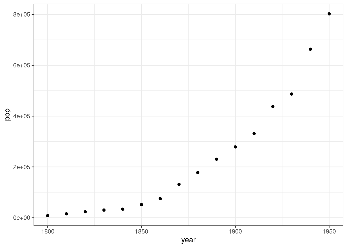

A researcher has determined that the following relationship approximates this growth well:

\[ \log(y) = -44.409 + 0.0299 x \]

Interpret the 0.0299 value.
Interpret the -44.409 value.
What is the average growth every 10 years?

Why use $e$ and not some other base?

Tradition.
For small values of $\beta_1$ (say, $-0.1 \leq \beta_1 \leq 0.1$), we can interpret $\beta_1$ as the proportion change for a 1 unit difference in $x$.
This is because for small $\beta_1$, we have $e^{\beta_1} \approx 1 + \beta_1$.

beta1	exp(beta1)	Percent Difference
0.00	1.000	0.000
0.02	1.020	2.020
0.04	1.041	4.081
0.06	1.062	6.184
0.08	1.083	8.329
0.10	1.105	10.517
0.12	1.127	12.750
0.14	1.150	15.027
0.16	1.173	17.351
0.18	1.197	19.722
0.20	1.221	22.140

In many real world applications, $\beta_1$ is typically small.
This relationship does not hold with other bases. E.g. $10^{0.02} = 1.0471 \not\approx 1 + 0.02$.
Example: From the DC population example above, we had $\beta_1 = 0.0299$ and $e^{\beta_1} = 1.0303$. So, a 3% larger population each year, and you can get that either from $\beta_1$ or $e^{\beta_1}$.

Power-law growth/decline

$\log(y) = \beta_0 + \beta_1 \log(x)$ represents power-law growth if $\beta_1 > 0$ and power-law decline if $\beta_1 < 0$.
- Sub-linear growth if $0 < \beta_1 < 1$.
- Super-linear growth if $\beta_1 > 1$.
Exponentiating both sides, we get the relationship \[ y = e^{\beta_0}x^{\beta_1} \]
Interpret $\beta_0$: The value of $y$ when $x = 1$ is $e^{\beta_0}$.
Interpret $\beta_1$:
- When you double $x$, you multiply $y$ by $2^{\beta_1}$.
- When you multiply $x$ by 10, you multiply $y$ by $10^{\beta_1}$.
- When you multiply $x$ by 1.1 (10% larger), you multiply $y$ by $1.1^{\beta_1}$.
- Choose a multiplier that makes sense for the range of your data. E.g., if it is never the case that one value is 10 times larger than another, don’t use that as the interpretation.
This follows from:

\[\begin{align} y_{old} &= e^{\beta_0}x^{\beta_1}\\ y_{new} &= e^{\beta_0}(2x)^{\beta_1}\\ &= e^{\beta_0}2^{\beta_1}x^{\beta_1}\\ &= 2^{\beta_1}e^{\beta_0}x^{\beta_1}\\ &= 2^{\beta_1}y_{old} \end{align}\]
Example: From the {Sleuth3} R package, we have a dataset on 7 islands measuring their land area and the number of species on each island. The goal is to estimate the relationship between these two variables, which has applications in conservation.
```
library(Sleuth3)
data("case0801")
ggplot(data = case0801, mapping = aes(x = Area, y = Species)) +
  geom_point()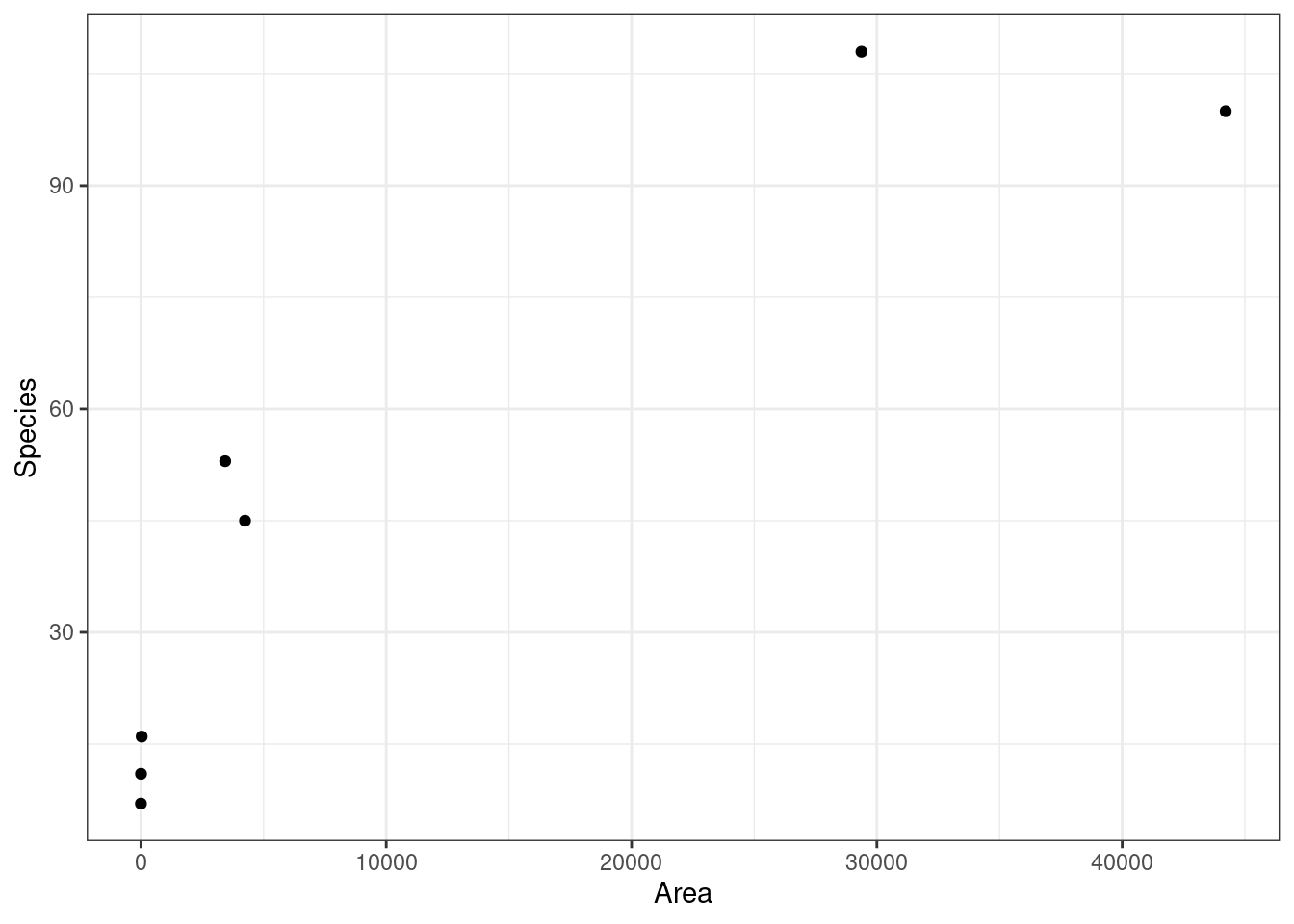
```
- This relationship is well-approximated by the curve $y = 6.9345x^{0.2497}$.
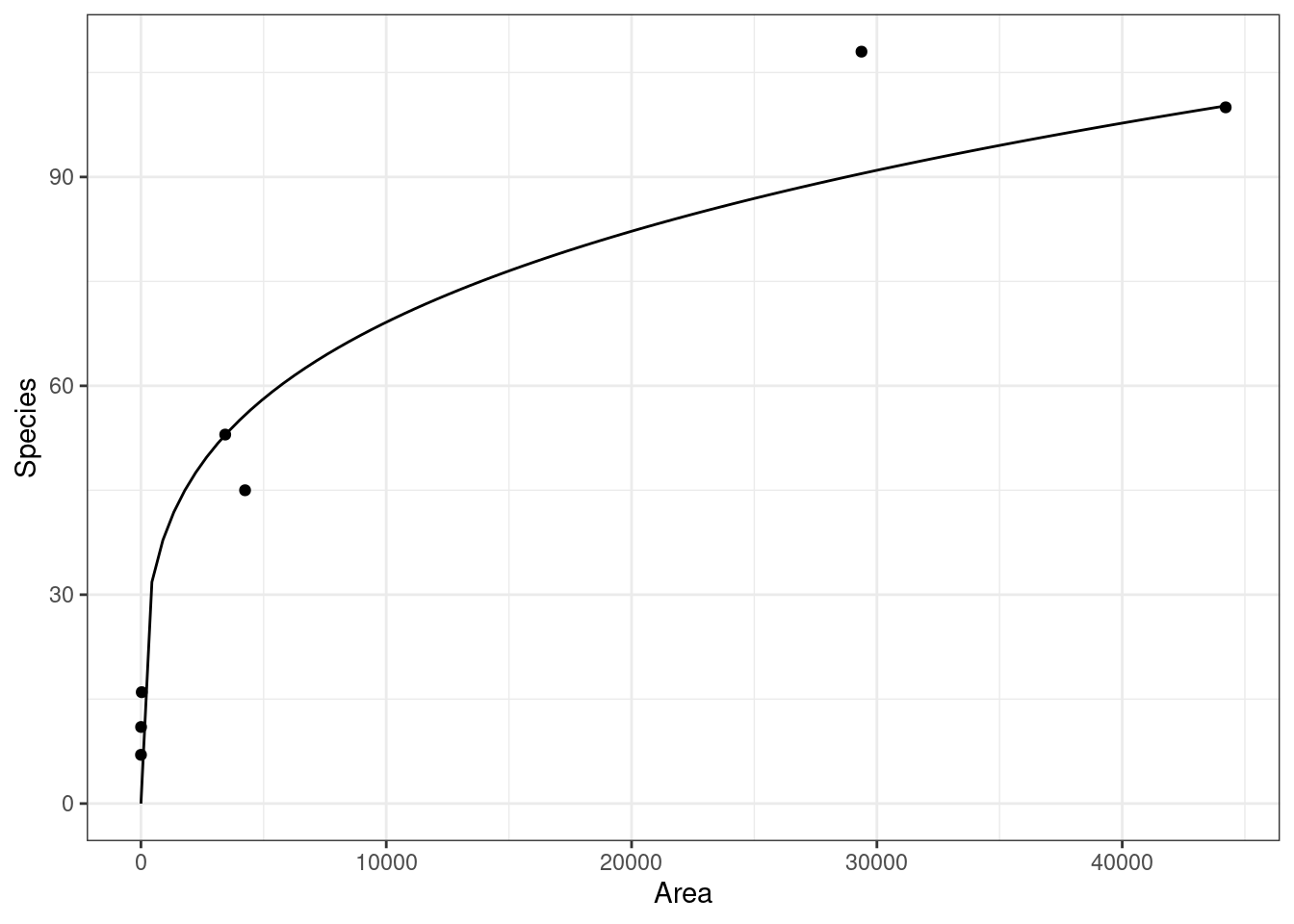
- So islands that are twice as large have $2^{\beta_1} = 2^{0.2497} = 1.1889$ times as many species on average. Or, islands that are twice as large have 19% more species on average.
- Notice that I didn’t use the language “change” or “increase”, because those would imply causal connections.
Exercise: Prove that the interpretation “when you multiply $x$ by 10, you multiply $y$ by $10^{\beta_1}$” is correct.
Exercise: Consider the wine consumption and heart disease data from the {Sleuth3} package. The observational units are the counties and the variables are
- Wine: consumption of wine (liters per person per year)
- Mortality: heart disease mortality rate (deaths per 1,000)
```
data("ex0823")
ggplot(data = ex0823, mapping = aes(x = Wine, y = Mortality)) +
  geom_point()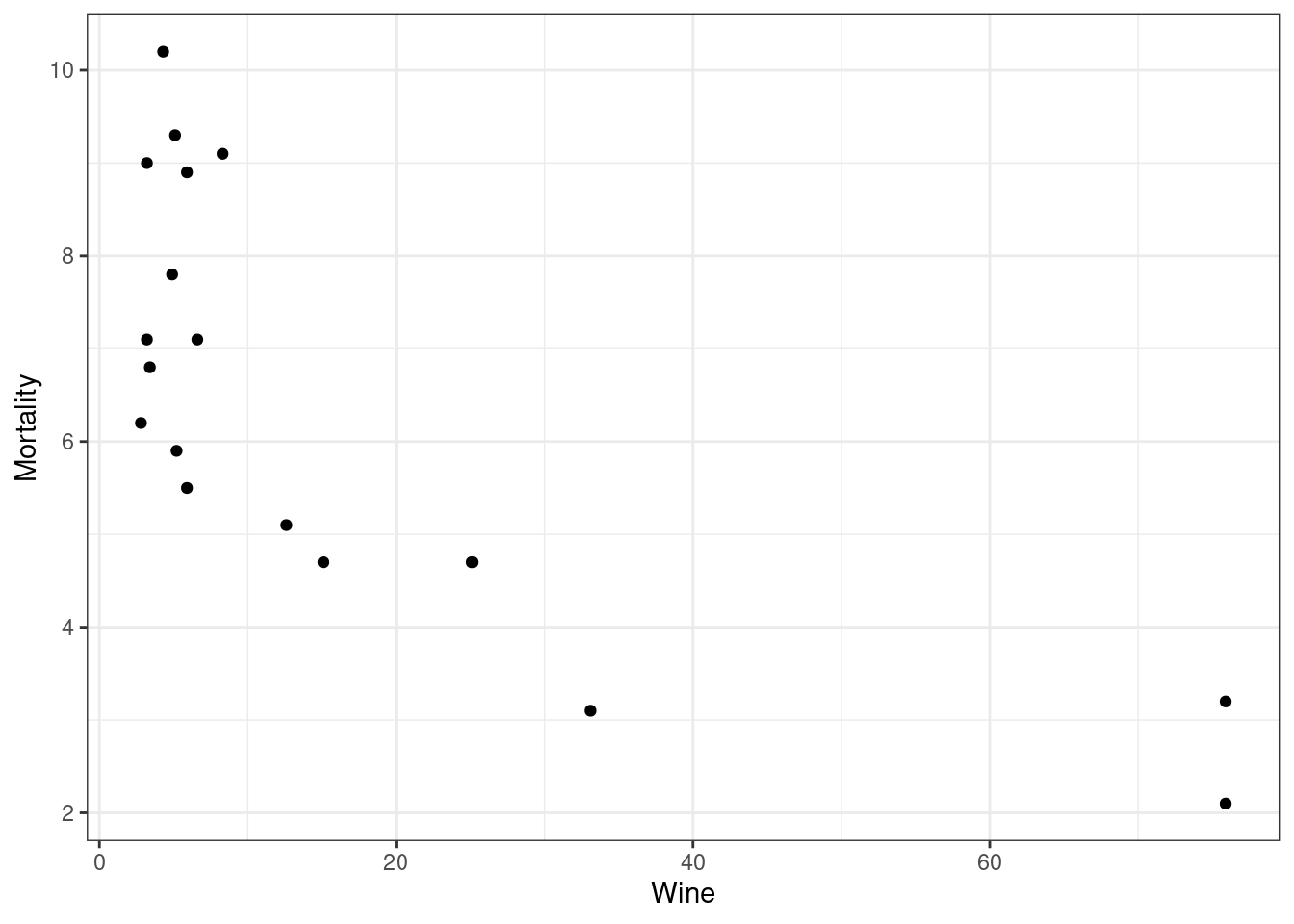
```
- Researchers have determined that this relationship is well-approximated by the following equation.
\[ y = 12.8784x^{-0.3556} \]
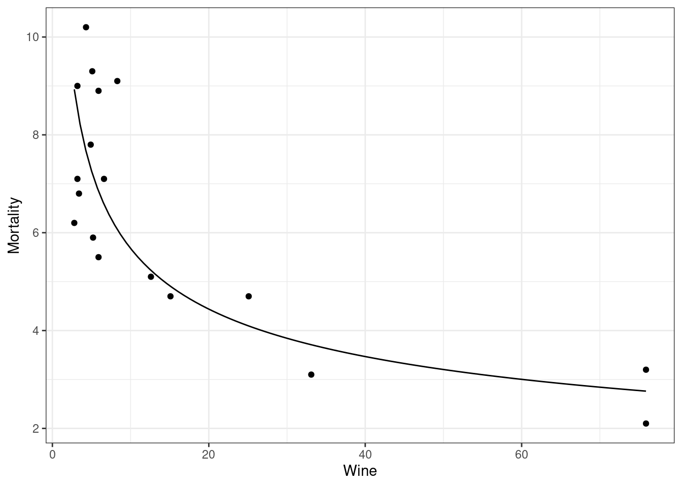
1. Interpret -0.3556.
2. Interpret 2.5556 (the value of $\beta_0$).
3. If one country drinks 50% more wine per person per year than another country, what is the expected difference in mortality rates?

Logging just the predictor variable

Sometimes, the relationship is of the form \[ y = \beta_0 + \beta_1 \log(x) \]
You intrepret $\beta_1$ with the following:
- When you double $x$, you add $\beta_1\log(2)$ to $y$.
- When you multiply $x$ by 10, you add $\beta_1\log(10)$ to $y$.
- When you multiply $x$ by 1.1 (10% larger), you add $\beta_1\log(1.1)$ to $y$.
- Choose a multiplier that makes sense for the range of your data. E.g. if it is never the case that one value is 10 times larger than another, don’t use that as the interpretation.
This follows from \[\begin{align} y_{old} &= \beta_0 + \beta_1\log(x)\\ y_{new} &= \beta_0 + \beta_1\log(2x)\\ &= \beta_0 + \beta_1[\log(x) + \log(2)]\\ &= \beta_0 + \beta_1\log(x) + \beta_1\log(2)\\ &= y_{old} + \beta_1\log(2). \end{align}\]

Example: From the mtcars dataset, it was determined that the relationship between mpg and wt was well approximated by the curve $y = 39.2565 + -17.0859\log(x)$.

df <- data.frame(x = seq(min(mtcars$wt), max(mtcars$wt), length.out = 100))
df$y <- beta0 + beta1 * log(df$x)
ggplot() +
  geom_point(data = mtcars, mapping = aes(x = wt, y = mpg)) +
  geom_line(data = df, mapping = aes(x = x, y = y))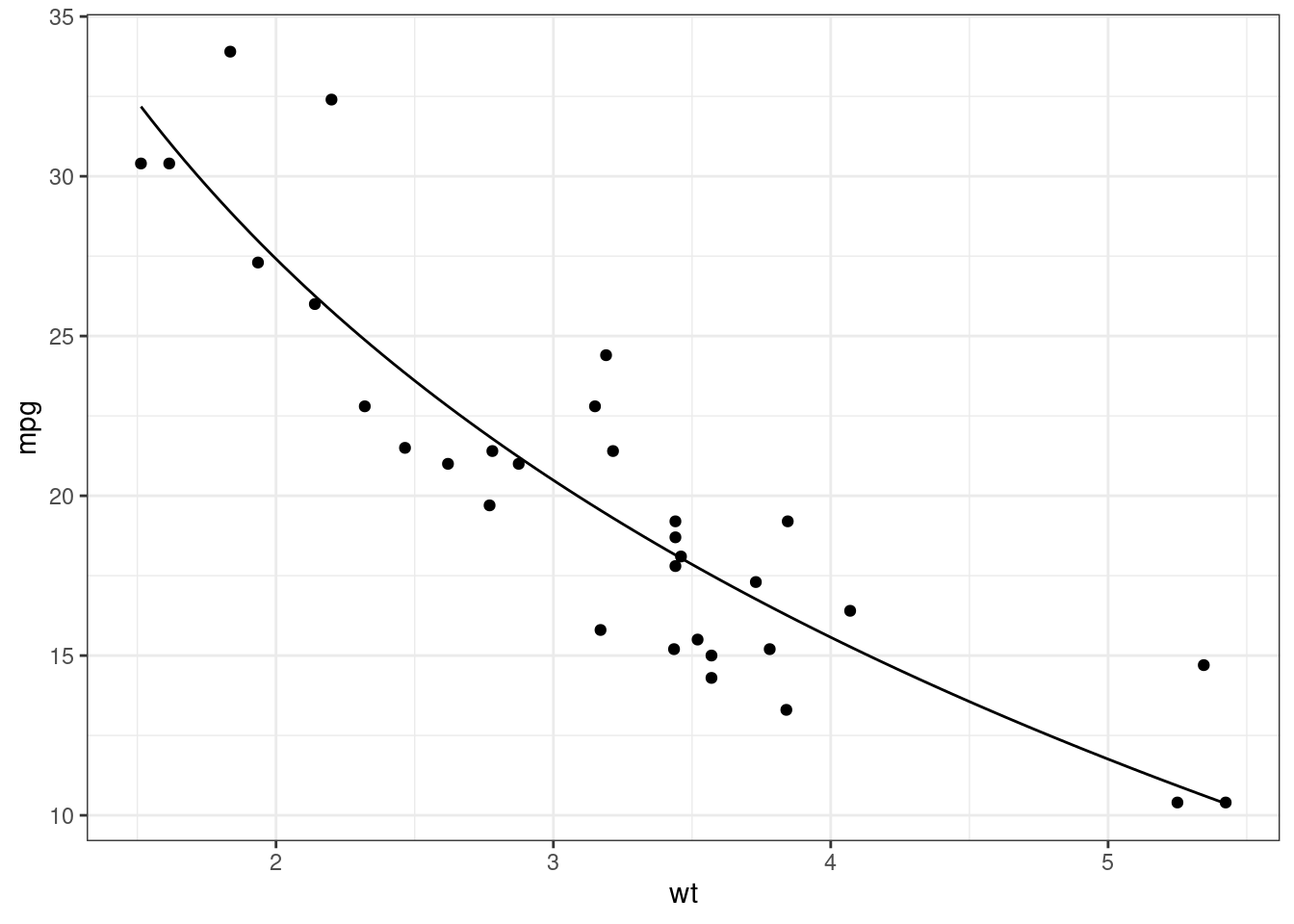

So cars that are 50% heavier have $-17.0 \times \log(1.5) = -6.9$ worse miles per gallon on average.

Summary of relationships on different scales

If relationship is $y = \beta_0 + \beta_1x$, then add $c$ to $x$ means add $c\beta_1$ to $y$.
If relationship is $y = \beta_0 + \beta_1 \log(x)$, then multiply $x$ by $c$ means add $\beta_1\log(c)$ to $y$.
If relationship is $\log(y) = \beta_0 + \beta_1 x$, then add $c$ to $x$ means multiply $y$ by $\exp(c\beta_1)$.
If relationship is $\log(y) = \beta_0 + \beta_1 \log(x)$, then multiply $x$ by $c$ means multiply $y$ by $c^{\beta_1}$.

Math Prerequisites

David Gerard

2024-01-23