Probability and Simulation
David Gerard
2024-01-23
Learning Objectives
- Basic Probability
- Normal/\(t\)-distributions
- Simulation in R
- Appendix A of KNNL.
Probability, the normal and \(t\) distributions.
A random variable is a variable whose value is a numerical outcome of a random process. We denote random variables with letters, like \(Y\).
In practice, this “random process” is sampling a unit from a population of units and observing that unit’s value of the variable. E.g., we sample birth weights of babies born in the United States, then birth weight a random variable.
The mean of a random variable is average value of a very large sample of individuals. The notation for the mean of a random variable is \(E[Y]\).
Properties:
- If \(a\) and \(b\) are constants (not random variables), then \(E[a + bY] = a + bE[Y]\).
- If \(X\) and \(Y\) are both random variables, then \(E[X + Y] = E[X] + E[Y]\).
The variance of a random variable is the average squared deviation from the mean of this random variable. It measures how spread out the values are in a population. The notation for the variance of a random variable is \(var(Y)\). Specifically \[ var(Y) = E[(Y - E[Y])^2] \]
Properties:
- If \(a\) and \(b\) are constants, then \(var(a + bY) = b^2var(Y)\)
The standard deviation of a random variable is the square root of its variance. \[ sd(Y) = \sqrt{var(Y)} \]
The distribution of a random variable is the possible values of a random variable and how often it takes those values.
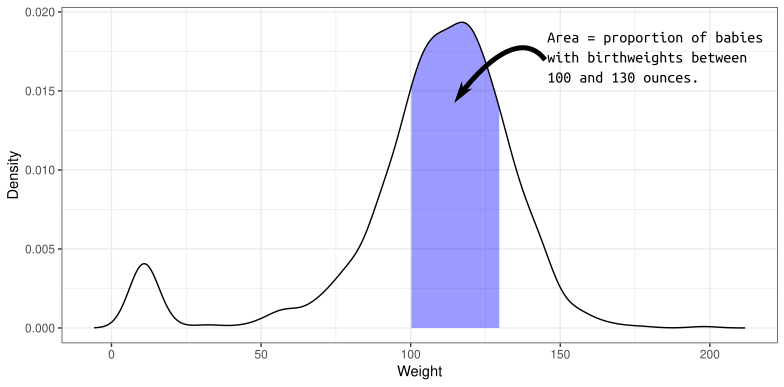
A density describes the distribution of a quantitative variable. You can think of it as approximating a histogram. It is a curve where
- The area under the curve between any two points is approximately the probability of being between those two points.
- The total area under the curve is 1 (something must happen).
- The curve is never negative (can’t have negative probabilities).
The density of birth weights in America:
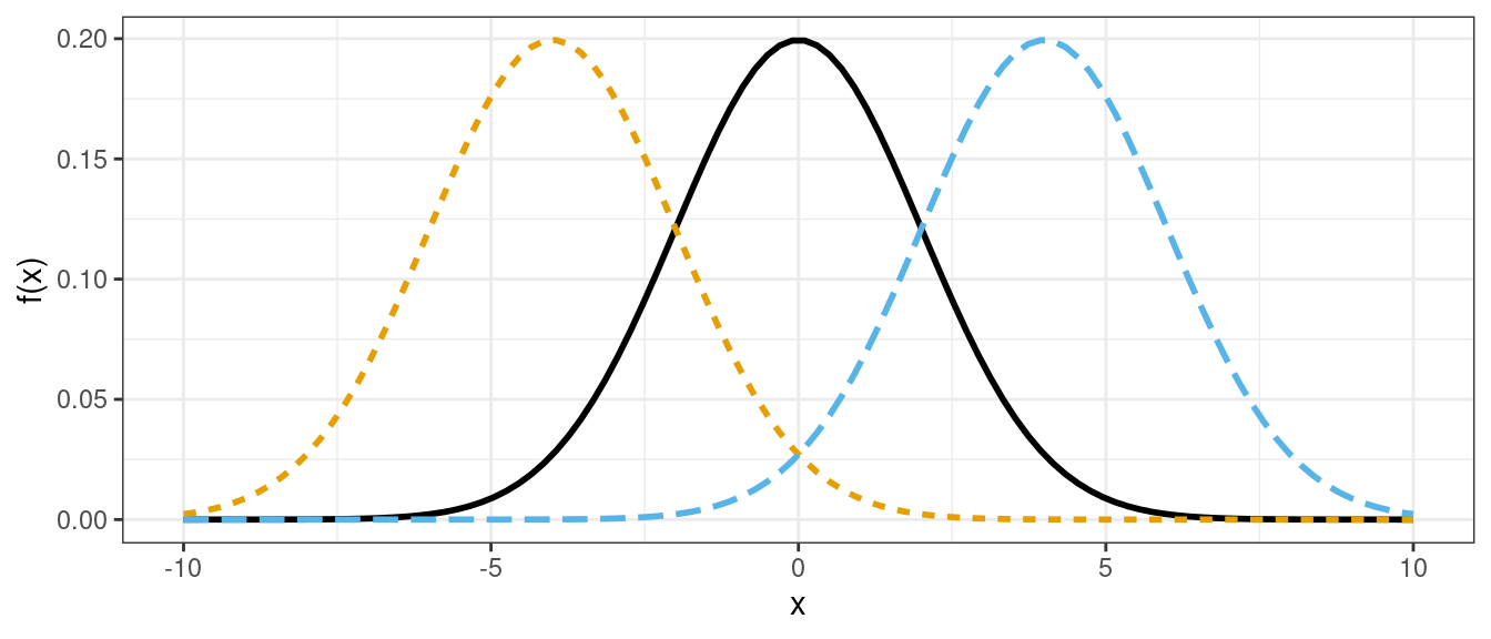
The distribution of many variables in Statistics approximate the normal distribution.
- If you know the mean and standard deviation of a normal distribution, then you know the whole distribution.
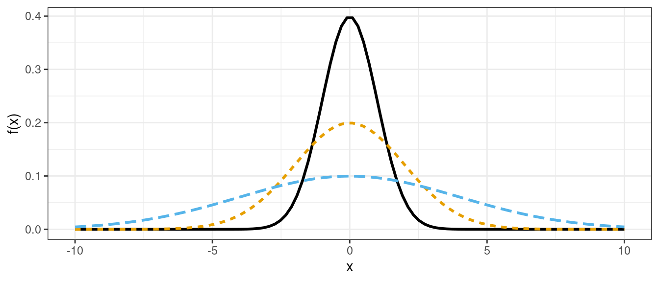
- Larger standard deviation implies more spread out (larger and smaller values are both more likely).
- Mean determines where the data are centered.
Normal densities with different means.
Normal densities with different standard deviations
Density Function (height of curve, NOT probability of a value).
dnorm(x = 2, mean = 1, sd = 1)## [1] 0.242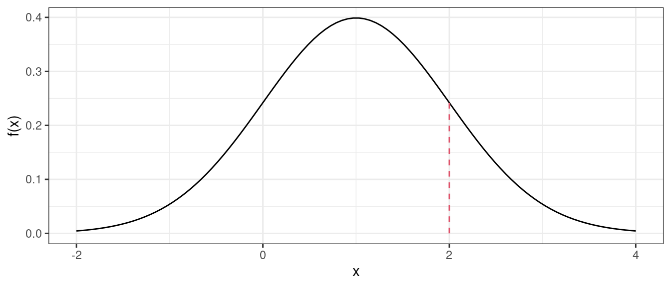
Random Generation (generate samples from a given normal distribution).
samp <- rnorm(n = 1000, mean = 1, sd = 1)
head(samp)
## [1] 0.03807 0.70747 1.25879 -0.15213 1.19578 1.03012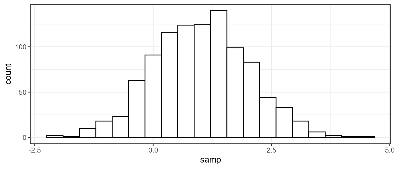
Cumulative Distribution Function (probability of being less than or equal to some value).
pnorm(q = 2, mean = 1, sd = 1)## [1] 0.8413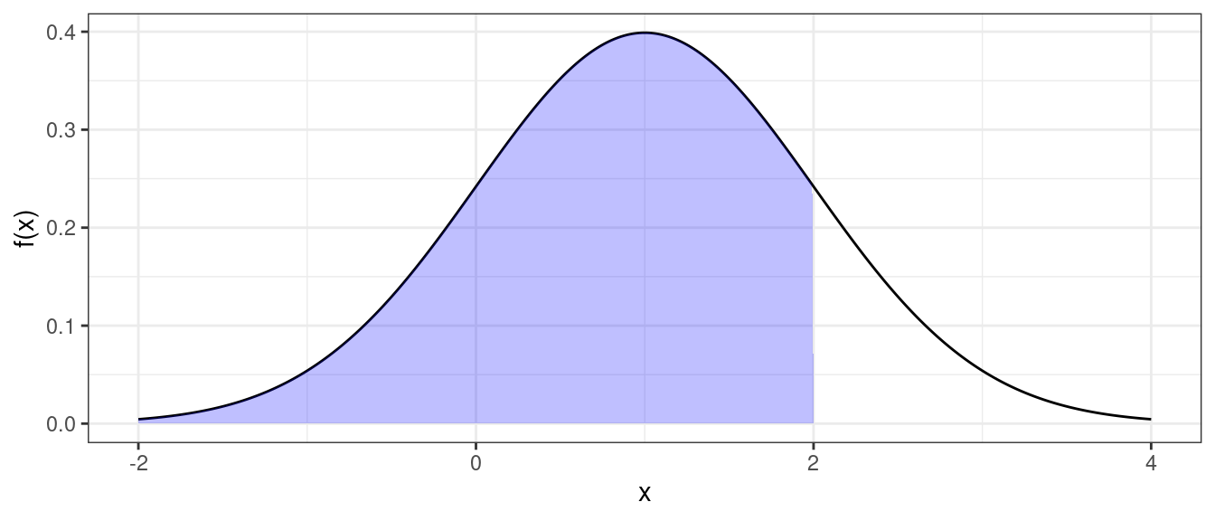
Quantile function (find value that has a given probability of being less than or equal to it).
qnorm(p = 0.8413, mean = 1, sd = 1)## [1] 2
Exercise: Use
rnorm()to generate 10,000 random draws from a normal distribution with mean 5 and standard deviation 2. What proportion are less than 3? Can you think up a way to approximate this proportion using a different function?Exercise: In Hong Kong, human male height is approximately normally distributed with mean 171.5 cm and standard deviation 5.5 cm. What proportion of the Hong Kong population is between 170 cm and 180 cm?
A property of the normal distribution is that if \(X \sim N(\mu, \sigma^2)\) and \(Z = (X - \mu) / \sigma\), then \(Z \sim N(0, 1)\).
Exercise: Use
rnorm()andqqplot()to demonstrate this property. That is, simulate 1000 values of \(X\) with some mean different than 0 and some variance different than 1. Then transform those \(X\) values to \(Z\). Then simulate some other variable \(W\) from \(N(0, 1)\). Useqqplot()to show that \(W\) and \(Z\) follow the same distribution.The \(t\)-distribution shows up a lot in Statistics.
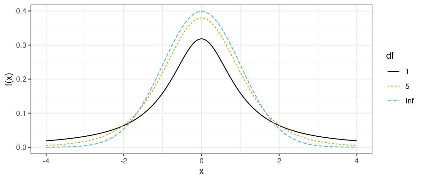
- It is also bell-curved but has “thicker tails” (more extreme observations are more likely).
- It is always centered at 0.
- It only has one parameter, called the “degrees of freedom”, which determines how thick the tails are.
- Smaller degrees of freedom mean thicker tails, larger degrees of freedom means thinner tails.
- If the degrees of freedom is large enough, the \(t\)-distribution is approximately the same as a normal distribution with mean 0 and variance 1.
\(t\)-distributions with different degrees of freedom:
Density, distribution, quantile, and random generation functions also exist for the \(t\)-distribution.
dt()
pt()
qt()
rt()
Covariance/correlation
The covariance between two random variables, \(X\) and \(Y\), is a measure of the strength of the linear association between these variables. It is defined as \[ cov(X, Y) = E[(X - E[X])(Y-E[Y])] \]
Covariance is related to correlation by \[ cor(X, Y) = \frac{cov(X, Y)}{sd(X)sd(Y)} \]